When we add or change some data in our data source, we need to refresh the pivot table to update the data in the pivot table. Sometimes, even after refreshing the page, the pivot table does not update, and the data remains unchanged. It might even show an error and refuse to refresh the pivot table. In this article, we will go through the reasons why the pivot table is not refreshing in your worksheet and provide solutions to all of those issues.
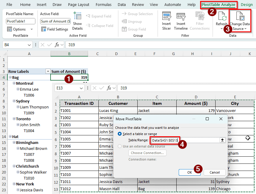
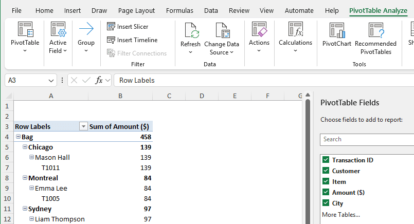
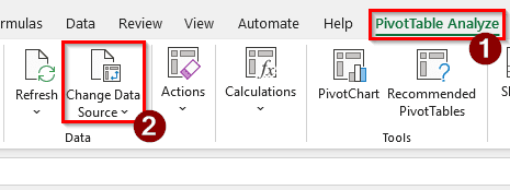
➤ Click on a cell of the pivot table and go to the PivotTable Analyze tab in the ribbon, and select Change Data Source from the Data section.
➤ Change the data source to add the new rows/columns for the pivot table.
➤ Press OK to confirm and check the pivot table for new data.
There could be a lot of reasons why the pivot table refuses to refresh properly. To learn about the possible solutions to those issues, read the full tutorial below.
Refreshing Does Not Add New Data to the Pivot Table
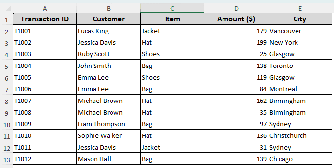
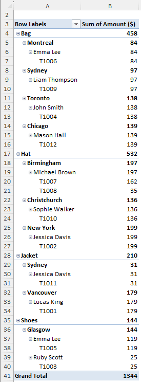
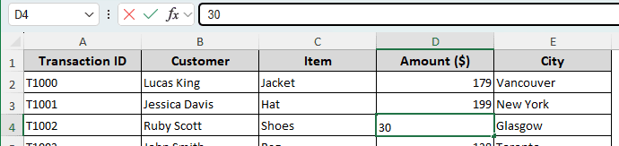
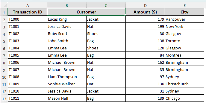
To demonstrate the issue, we have a data range with some retail transactions data. There are transaction IDs, customer names, sold items, the amount of money earned from selling those items, and the cities those items were shipped to.

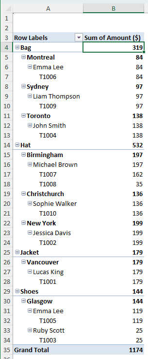
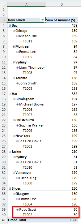
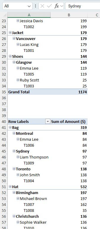
Then we created a pivot table using the data, which looks like this:
Let’s add some more data and refresh the pivot table.
➤ After those 10 transactions, two more transactions happened. We added those in the source data table.
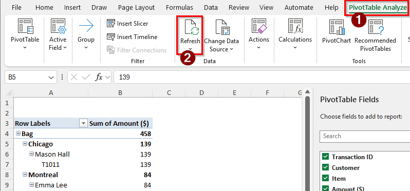
➤ Now let’s right-click on the pivot table and hit Refresh.
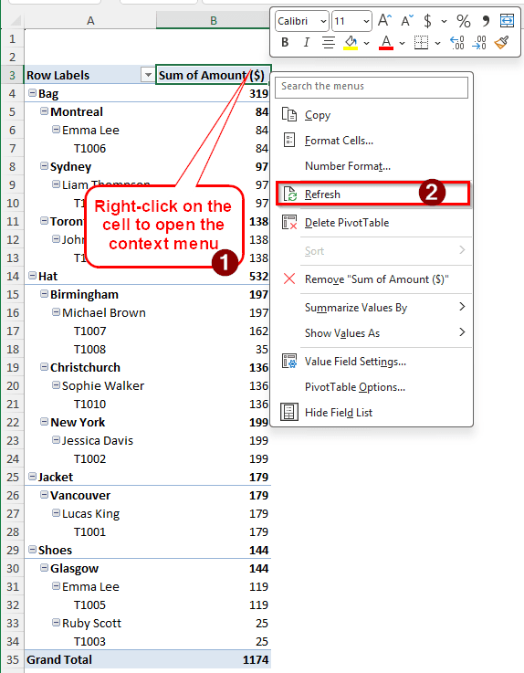
➤ However, the pivot table remains the same, and the new transactions are not included. We have to fix that.
Solution 1: Use a Proper Table as the Data Source
The issue is that when we created the pivot table, we only selected the entries that were recorded at that time. The pivot table will only look through the cells that it is aware of, not the new cells that we add. To overcome this issue, we can convert the source dataset to a table. Then, when we add new data to the table, the table will be updated, and the pivot table will follow the regular table.
➤ Select the source dataset and press Ctrl + T .
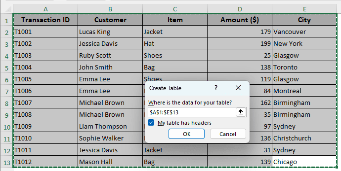
➤ Press OK to create the table.
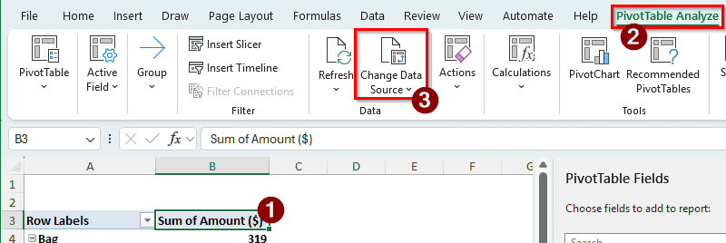
➤ Now go to the pivot table and select a cell so that we can customize the table.
➤ Find the PivotTable Analyze tab in the ribbon, and click on Change Data Source from the Data group.
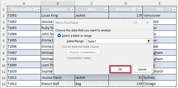
➤ Select the table (Named Table1 in this case) and press OK.
➤ Now the pivot table should be updated with the new data. Next time you add more data to the table, the pivot table will include it as well when you refresh it.
Solution 2: Use a Data Name
If we don’t want to create a regular table, we can create a data name that we will use as a variable for the pivot table. We will need to use a function for that as well. Follow the steps below:
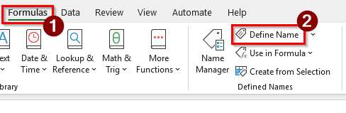
➤ In the sheet where the source dataset belongs, go to the Formulas tab and select Define Name from the Defined Names group.
➤ In the Name section, write Dataset, and in the Refers to section, write the following formula:
=OFFSET(Data!$A$1,0,0,COUNTA(Data!$A:$A),COUNTA(Data!$1:$1))
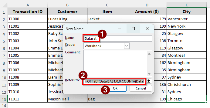
➤ Press OK to add the Name.
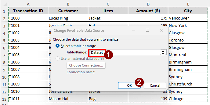
➤Go to the pivot table, and head to PivotTable Analyze > Change Data Source. Then, change the source to Dataset.
➤ From now on, the pivot table will refresh properly after you add anything to your dataset.
Refreshing Does Not Change the Existing Data
We know that a pivot table will not pull new data if not specified, but it should refresh the existing data. However, that might not be the case every time. See the example below:
➤ We are changing the D4 cell, and making the Amount 30 instead of 25.
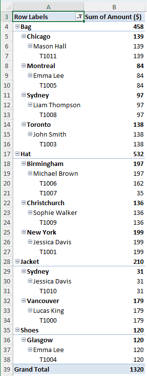
➤ Moving back to the pivot table and pressing Alt + F5 does nothing; the transaction is not visible.
Solution: Remove the Filters
The fix for the issue is just removing the filters. It had filters that did not let the target cell be shown in the pivot table. We need to remove the filters to see the changes.
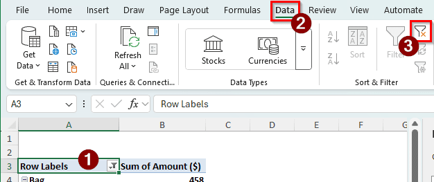
➤ When you have the pivot table selected, go to the Data tab in the ribbon.
➤ From the Sort & Filter group, select the Clear button.
➤ Now the changes are visible on the pivot table.
PivotTable Field Name is Not Valid
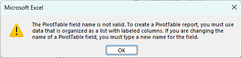
While refreshing the pivot table, Excel can throw an error that says “The PivotTable field name is not valid”. Check the demonstration below:
➤ Go to the PivotTable Analyze tab and select Refresh from the Data group.
➤The following error should show up:
Solution 1: Check for Column Errors
There could be two issues in the columns of the source data. We will fix both of them in this section.
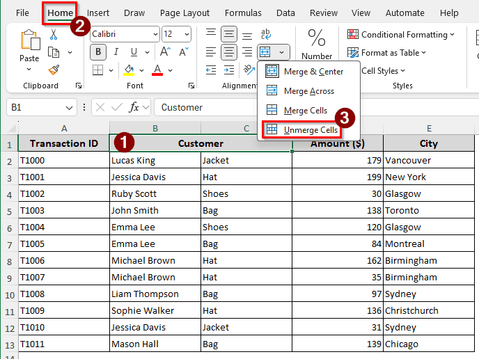
➤ One issue could be that the column headers are merged. Look at the following image:
➤ While you have the cell selected, go to the Home tab, and select Unmerge Cells from the Alignment group.
➤ Another issue could be that the column header went missing for some reason, like the image below:
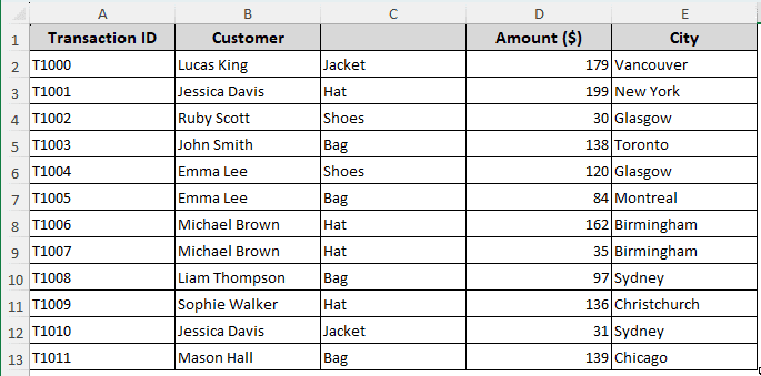
➤ For this case, the issue is that we had a merged cell, and after unmerging, we have to restore the header to fix this issue.
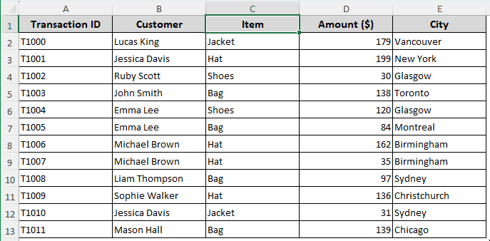
➤ Now, if you refresh the pivot table, it will work properly.
Solution 2: Look for Missing Data Source
Another issue can be that the data that was used to create the pivot table is missing. You have to restore the data to the original location to fix the issue.
➤ Go to PivotTable Analyze > Change Data Source.
➤ Now, the pivot table will show you where your data is supposed to be:
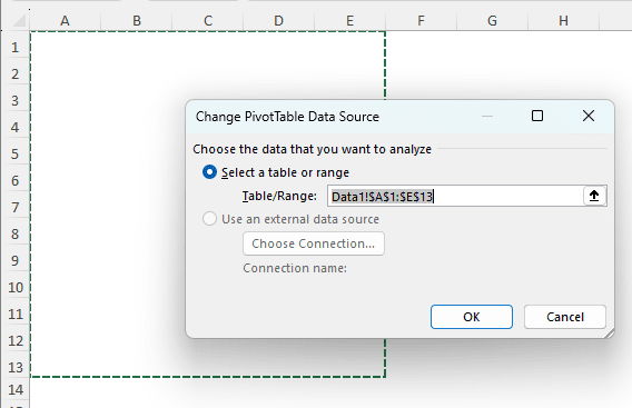
➤ Add the data to this source, or change the source to get the pivot table working again.
Overlapping Pivot Tables
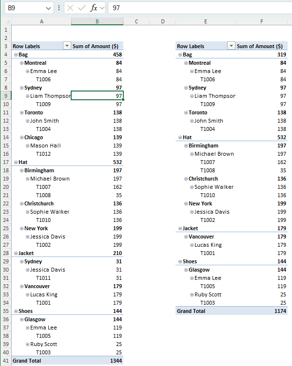
In order to show what the issue can look like, we are adding two pivot tables in the same sheet.
➤ After adding more transactions to the first table, try to refresh it by pressing Alt + F5 . The following error should show up:
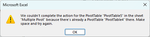
➤ The issue is that the pivot tables are overlapping with each other when the data is updated. We cannot have one pivot overlapping another.
Solution: Move the Pivot Table to Another Place
We need to move the second pivot table to a location where it cannot cause conflict with another one. Follow the steps below:
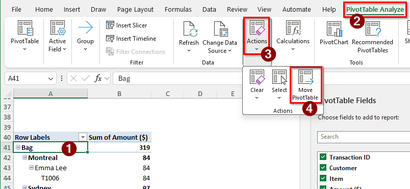
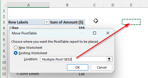
➤ Select the pivot table that is below the original table, and go to PivotTable Analyze > Actions > Move PivotTable
➤ Select a different location and press OK.
➤ Now, if you refresh the pivot table, it will work properly.
Frequently Asked Questions
Why is my PivotTable still showing old data?
Whenever you add new data to your source dataset, you must refresh the pivot table to make the new data show up. Pivot tables do not automatically refresh each time you add data to the source table. However, you can set it to refresh every time you open your workbook.
Why is my PivotTable not showing totals?
The totals are probably hidden from the pivot table. You can enable them by going to the Design tab in the pivot table and finding the Subtotals and Grand Totals icons from the Layout group. Choose Show all Subtotals at Bottom/Top of Group and On for Rows and Columns.
How to reset PivotTable data?
Click on the pivot table, and go to the PivotTable Analyze tab on the ribbon. Then, from the Actions group, choose Clear > Clear All. The pivot table will be reset, and you can customize the table as a new one.
Why don’t pivot tables update automatically?
In most cases, pivot tables are created with a lot of CSV data. If the pivot table is updated automatically when the real-time CSV data changes, it would be impossible to work with the pivot table because of the changes. Moreover, the worksheet will be laggy because it has to process everything in the background. That is why pivot tables are not updated automatically.
How to update a PivotTable with new columns?
Go to the PivotTable Fields panel and select the new columns from the checklist. You can also drag the columns to the specific areas at the bottom. If the panel does not show up, right-click on the pivot table and select Show Field List.
Wrapping Up
In this article, we have learned all possible issues and solutions regarding pivot tables not refreshing. If you have more difficulties dealing with the pivot table refresh situation, let us know in the comments section. Don’t forget to download the practice file provided with the article. See you soon in another article.