The VLOOKUP function is one of Excel’s most useful tools for finding information, but not every search will return an exact match. In many cases, your lookup value may fall between two entries, such as an income bracket, a grade cutoff, or a discount range. This is where using the VLOOKUP function to find the closest match becomes important.
With approximate match, VLOOKUP function doesn’t just look for exact values. Instead, it searches your table and returns the closest value that is less than or equal to the number you enter. This makes it a practical solution for calculating tax rates, assigning grades, or applying tier-based pricing.
In this article, we’ll show you how to use the VLOOKUP function to find the closest match using some simple methods.
Here’s how to use VLOOKUP function to find the closest match in Excel:
➤ Open your dataset in Excel.
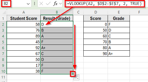
➤ Select cell B2 next to the first student score.
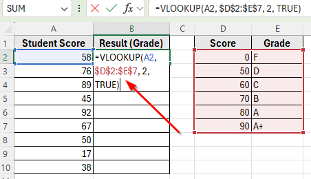
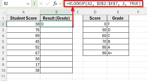
➤ Enter the formula: =VLOOKUP(A2, $D$2:$E$7, 2, TRUE)
➤ Press Enter. Excel will return the correct grade based on the nearest score.
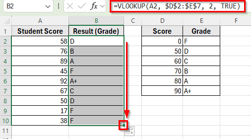
➤ Drag the fill handle down from cell B2 to B10 to apply the formula to the other student scores.
Applying VLOOKUP Function to Find the Closest Approximate Match
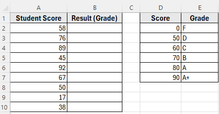
In the following dataset, Column A contains Student Scores, and Column B labeled as Result (Grade) which is currently empty. On the right, Column D has Scores, and Column E lists the Grades.
Our goal is to use the VLOOKUP function with an approximate match to return the correct grade into Column B.
We’ll use this dataset to demonstrate how the VLOOKUP function with approximate match works in Excel.
The VLOOKUP function has a built-in option to return the closest match if the exact value isn’t found. By setting the fourth argument to TRUE, Excel looks for the nearest value less than or equal to your lookup value.
Here’s a simple step by step guide to apply this method:
➤ Open your dataset in Excel.
➤ Select cell B2 next to the first student score.
➤ Enter the formula:
=VLOOKUP(A2, $D$2:$E$7, 2, TRUE)
➤ Press Enter. Excel will return the correct grade based on the nearest score.
➤ Drag the fill handle down from cell B2 to B10 to apply the formula to the other student scores.
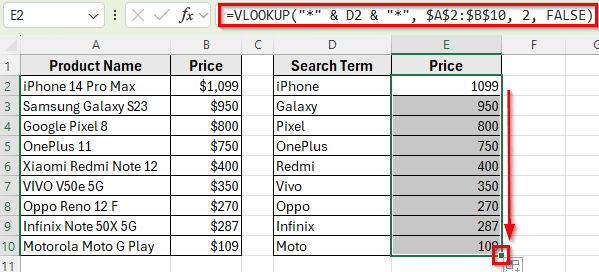
Using VLOOKUP Function to Find a Partial Text Match
In the following dataset, Column A contains Product Names, and Column B shows their corresponding Prices. On the right, Column D has Search Terms that include only part of the product name.
Our goal is to use VLOOKUP with a wildcard to return the matching product price into Column E.
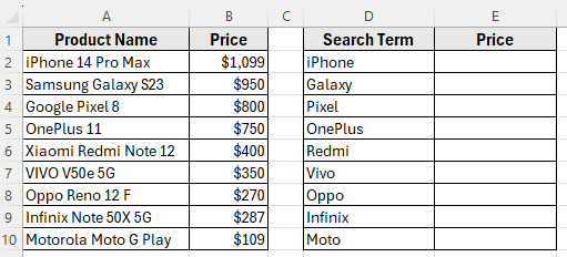
Sometimes you don’t have the exact text in your lookup value. For example, you might have only part of a product name or keyword, but still want to pull out the related information. By combining with wildcard characters, you can find and return results based on a partial text match.
Here’s how to apply this method:
➤ Open your dataset in Excel.
➤ Click on cell E2 next to the first search term.
➤ Enter the formula:
=VLOOKUP("*" & D2 & "*", $A$2:$B$10, 2, FALSE)
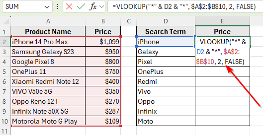
➤ Press Enter. Excel will return the correct price of the product containing the word iPhone.
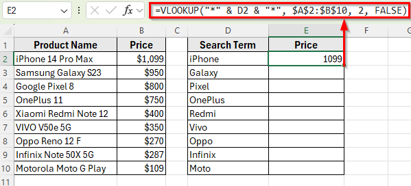
➤ Drag the fill handle down from E2 to E10 to copy the formula for the rest of the search terms.
Note:
When using VLOOKUP with wildcards such as asterisk or question mark, Excel only shows the first match. If there are multiple similar results, it won’t display them all, just the first one it finds.
Frequently Asked Questions
What is the difference between exact and approximate match in VLOOKUP?
Using FALSE returns an exact match only. If the lookup value doesn’t exist, you get an #N/A error. With TRUE, the VLOOKUP function looks for the closest value less than or equal to your lookup entry. For this to work correctly, your lookup column must be sorted in ascending order.
How do I fix VLOOKUP returning #N/A with an approximate match?
Usually, this happens because your lookup value is smaller than the smallest value in the lookup table, or the first column isn’t sorted. Make sure the data is sorted ascending and your lookup value lies within the range.
What does VLOOKUP do in Excel?
The VLOOKUP function searches for a value in the first column of a table and returns a related value from another column in the same row. It’s one of Excel’s most common lookup tools.
Wrapping Up
The VLOOKUP function can do much more than just find exact values. You can also use it to find the closest number, check ranges like tax or commission, or match part of a text using wildcards.
The important part is choosing the right match type. Exact match is best when you want precise results, while approximate match helps when your data is range based. If your table is sorted properly, the VLOOKUP function can simply return the nearest result and make your calculations easier.
With these methods, you can handle different tasks in Excel more easily, from grading and discounts to pricing and reports.