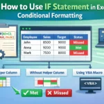
With Excel’s Conditional Formatting feature, you can apply formatting (e.g., color fills, font changes, or borders) to cells based on specific rules. Excel’s built-in Text That Contains option only works for one specific text string.
For more flexibility and better control, you can use a simple formula instead with functions like ISTEXT, AND, OR, EXACT, etc. Besides finding specific texts and partial searches, formula-based formatting allows you to highlight based on multiple conditions, exclude blanks, highlight duplicates, check text length, use dynamic lists for matching, and more.
➤ Click and drag to select your data range, go to the Home tab, and select the Conditional Formatting drop-down. Choose New Rule from the menu
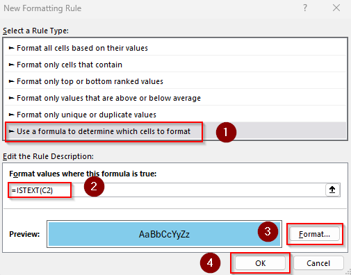
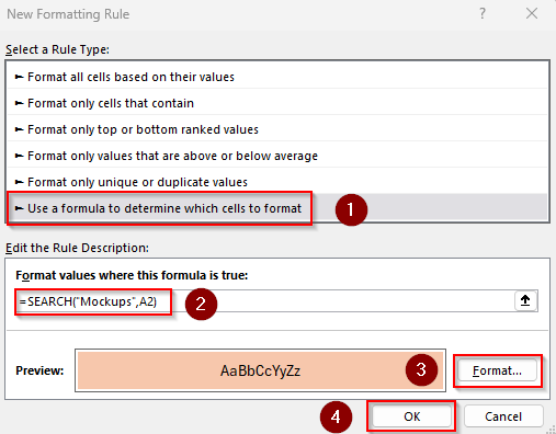
➤ As the New Formatting Rule dialog box opens, click the Use a Formula to Determine Which Cells to Format option.
➤ In the Format Values Where This Formula Is True box, insert the following formula to highlight any cell containing text: =ISTEXT(C2)
➤ C2 is the first cell of our range. Change the reference, set your desired formatting, and click Ok.
This article covers the ways of setting formula-based conditional formatting rules for texts with functions like ISTEXT, SEARCH, AND, OR, COUNTIF, and FIND.
Apply Conditional Formatting Formula for Cells Containing Specific Text
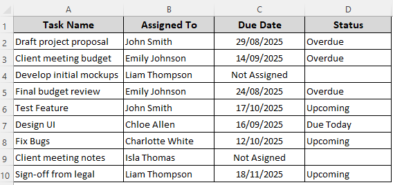
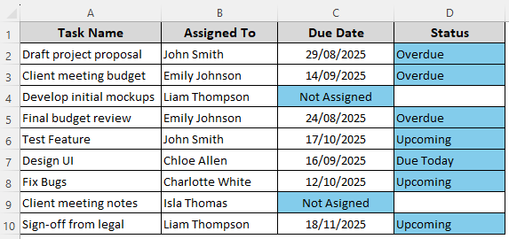
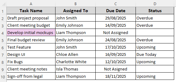
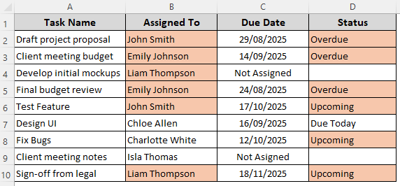
Our sample dataset has columns for project tasks, assignee names, due dates, and current status. For projects without a due date, Column C says Not Assigned and the corresponding cells in Column D are blank.
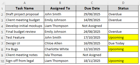
We aim to highlight the cells containing the text Upcoming. You can use it directly in the formula or enter it in cell F2 and use it as a reference in the formula. Here are the steps for it:
➤ Select the data range you want to format and open the Home tab. From the Styles group, click on the Conditional Formatting drop-down. Choose New Rule from the menu.
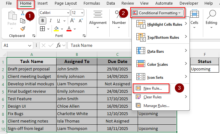
➤ Excel will now open the New Formatting Rule dialog box. From the Select a Rule Type group, scroll down and select Use a Formula to Determine Which Cells to Format.
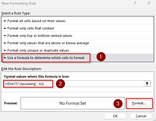
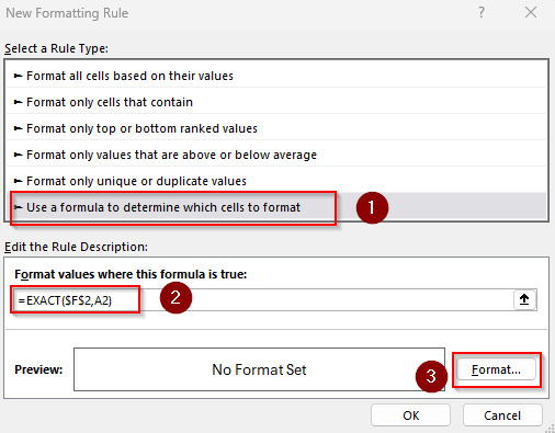
➤ In the Format Values Where This Formula Is field, type any of the following formulas:
Formula with Text
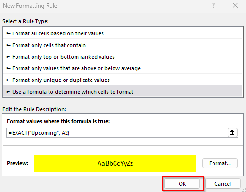
=EXACT("Upcoming", A2)
Formula with Cell Reference
=EXACT($F$2,A2)
➤ Here, A2 is the first cell of our range and F2 contains the lookup text. Change them according to your dataset. Keep in mind that this formula is case sensitive (doesn’t ignore capitalization).
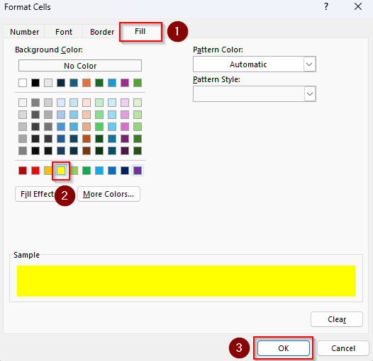
➤ Press the Format button and choose your preferred formatting by setting the Number, Font, Border, or Fill. Click Ok when you’re done.
➤ Press Ok to close the New Formatting Rule dialog box.
➤ Here’s the final result:
Format Cells Containing Any Text
To highlight cells that only contain text (not numbers, signs, or errors), follow the steps given below:
➤ Select your data range (C2:D10 for our dataset) and click on the Home tab >> Conditional Formatting drop-down >> New Rule >> Use a Formula to Determine Which Cells to Format.
➤ In the Format Values Where This Formula Is True box, enter this formula:
=ISTEXT(C2)
➤ Change the first cell of the range C2 as needed.
➤ Now, click on Format and choose your preferred formatting style. Press Ok.

➤ Click Ok to see the result as shown below:
Conditional Formatting Formula for Partial Matches
With the SEARCH and FIND functions, you can highlight partial matches. For example, if you enter Mock in the formula, it will highlight the cell containing the text Mockups. Use SEARCH for case-insensitive matches and FIND for case-sensitive lookups. Below are the details:
➤ Select your data range and go to the Home tab >> Conditional Formatting drop-down >> New Rule >> Use a Formula to Determine Which Cells to Format.
➤ Click on the Format Values Where This Formula Is True field and insert any of the following formulas:
For Case-Insensitive Matches
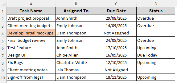
=SEARCH("Mockups",A2)
➤ Replace A2 with the top-left cell reference of your range.
➤ Use the Format button to set formatting rules and press Ok.
➤ Close the dialog box by pressing Ok and see the result.
For Case-Sensitive Matches
=FIND("mockups",A2)
➤ Change the cell reference A2 as needed.
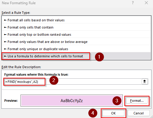
➤ Set the formatting rules, press Ok, and check the final output:
Highlight Cells with Text of a Certain Length
If you want to highlight text only if it has a specific number of characters, follow these steps:
➤ Select the range containing the cells you want to highlight and click on the Select your data range and click on the Home tab >> Conditional Formatting drop-down >> New Rule >> Use a Formula to Determine Which Cells to Format.
➤ Type the following formula in the Format Values Where This Formula Is True box:
=AND(ISTEXT(A2),LEN(A2)=10)
➤ This formula highlights cells that contain exactly 10 characters of text. Replace 10 with any number you need and change A2 to the first cell of your range.
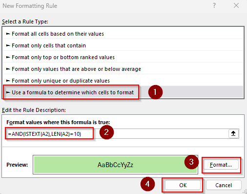
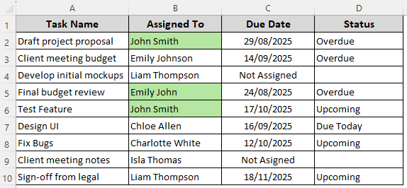
➤ Set the formatting rules using the Format option and press Ok. After formatting, our dataset looks like this:
Format Cells That Contain One of Multiple Text Values
Use this method if you want to highlight if a cell contains any one of several words. Here, we’ll highlight cells containing Client, Budget, or Meeting. Let’s get to the steps:
➤ Click and drag to select your data range and go to the Home tab >> Conditional Formatting drop-down >> New Rule >> Use a Formula to Determine Which Cells to Format.
➤ Select the Format Values Where This Formula Is True box and insert this formula:
=OR(ISNUMBER(SEARCH("Client",A2)),ISNUMBER(SEARCH("Meeting",A2)),ISNUMBER(SEARCH("Budget",A2)))
➤ To match your dataset, replace A2 with the first cell of your selected range. Also, you can change the words and add or reduce them as needed.
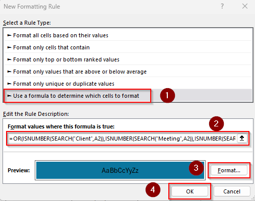
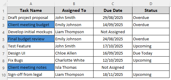
➤ Choose your preferred format using the Format option and press Ok. Here’s the final result:
Format Cells That Contain All of Multiple Text Values
In this case, our formula will highlight a cell only if it contains Client, Meeting, and Budget together in a text string. Below are the steps:
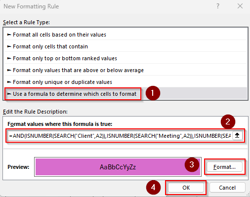
➤ Choose and highlight your range and open the Home tab >> Conditional Formatting drop-down >> New Rule >> Use a Formula to Determine Which Cells to Format.
➤ Under the Format Values Where This Formula Is True option, enter this formula in the box:
=AND(ISNUMBER(SEARCH("Client",A2)),ISNUMBER(SEARCH("Meeting",A2)),ISNUMBER(SEARCH("Budget",A2)))
➤ Replace the values and cell references as needed.
➤ Choose formatting options and press Ok to close the dialog box.
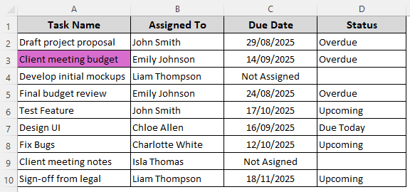
➤ Below is our formatted dataset:
Conditional Formatting Formula for Duplicate Texts
To highlight texts that occur more than once, follow the steps given below:
➤ Select the cell range containing the duplicates and click on the Home tab >> Conditional Formatting drop-down >> New Rule >> Use a Formula to Determine Which Cells to Format.
➤ Insert the following formula in the Format Values Where This Formula Is True field:
=COUNTIF($A$2:$D$10,A2)>1
➤ Here, $A$2:$D$10 is our data range and A2 is its first cell. Replace these references according to your dataset.
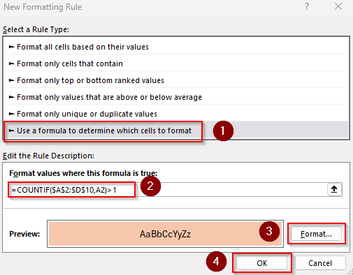
➤ Set the formatting rules and click Ok to see the final result.
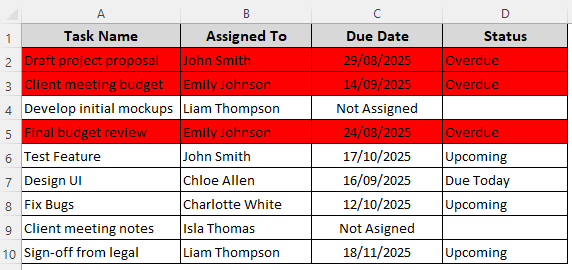
Formatting the Entire Row Based on the Text Result
Here, we’ll highlight the entire row when a certain text is found in any cell of the row. In our dataset, we are formatting the row in light red if the deadline is Overdue. Here’s how:
➤ Select the entire data range and open the Home tab >> Conditional Formatting drop-down >> New Rule >> Use a Formula to Determine Which Cells to Format.
➤ In the Format Values Where This Formula Is True box, insert this formula:
=$D2="Overdue"
➤ $D2 is the first cell of the column containing the value Overdue. Change the cell reference and value as required.
➤ Click Format and choose your preferred formatting options. Press Ok.
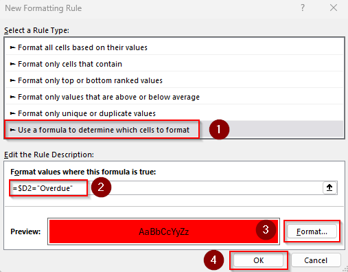
➤ Close the dialog box by pressing Ok. Check the final result.
Frequently Asked Questions
How to change cell color in Excel based on text input automatically?
To automate the highlighting process for specific texts, go to theHome tab >> Conditional Formatting drop-down >> New Rule >> Use a Formula to Determine Which Cells to Format. In the formula box, enter:
=A2="Completed"
Replace A2 with the first cell of your range and set your preferred formatting style. You can add more rules for more specific texts following the same process.
How to use conditional formatting in Excel based on text in another cell?
If you want to format one cell/range based on the text in another cell, lock the reference with $. For example, if you want to highlight the cells of Column A when Column C has “Completed”, highlight Column A (A2:A10) and open the Home tab >> Conditional Formatting drop-down >> New Rule >> Use a Formula to Determine Which Cells to Format. In the designated field for the formula, insert:
=$B2="Completed"
Format as you prefer, and the entire Column A will change based on Column B’s text.
How to highlight cells beginning or ending with specific text?
To highlight cells where text starts or ends with certain characters, use LEFT or RIGHT functions in conditional formatting. When setting the formatting rules, use this formula to find the text beginning with INV:
=LEFT(A2,3)="INV"
Format the text ending with Ltd using this formula:
=RIGHT(A2,3)="Ltd"
Change the texts, and the first cell of the range A2 based on your dataset.
Concluding Words
While applying conditional formatting rules, make sure texts, dates, and numbers are formatted correctly according to Excel’s formatting styles. Otherwise, Excel might recognize numbers and dates as text. To edit or delete the conditional formatting formulas, go to the Home tab >> Conditional Formatting >> Manage Rules.