In general, Excel’s conditional formatting is used to highlight a cell based on its own value. However, you can use a formula to format an entire column based on the value of a different column. It allows you to highlight a cell if a different cell contains a certain text or numeric value.
You can use the AND and OR functions to combine multiple conditions and highlight cells when those conditions are met.
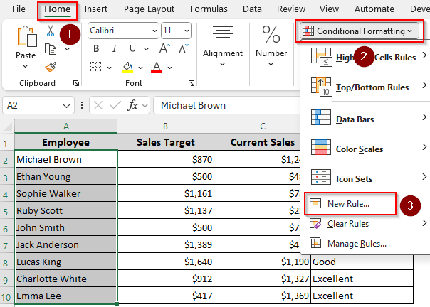
➤ Select the column cells where you want to apply the formatting rule. From the Home tab, click on the Conditional Formatting drop-down and select New Rule.
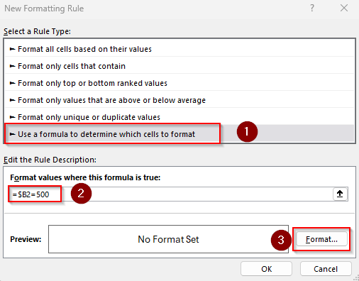
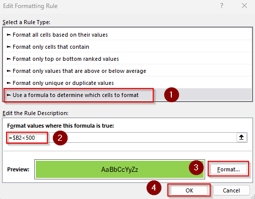
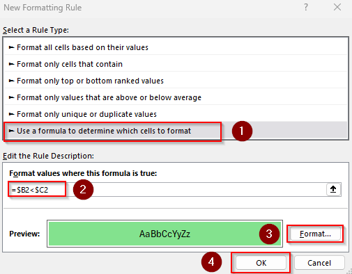
➤ When the New Formatting Rule dialog box appears, choose the Use a Formula to Determine Which Cells to Format option.
➤ In the Format Values Where This Formula Is True box, insert the following formula to highlight cells in Column B if the values in Column B are less than the corresponding values in Column C:
=$B2<$C2
➤ $B2 and $C2 are the first cells of Columns B and C without the headers. Change the values according to your dataset.
➤ Press the Format button to choose formatting options and click Ok Close the dialog box by pressing Ok to apply the formatting rule.

Apart from this rule, we’ll cover more formatting formulas to highlight a column when the values of a different column are equal, greater, or less than a certain value. We’ll also highlight based on text values and multiple conditions.
Format Based on Numerical Values in Another Column
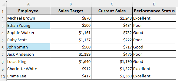
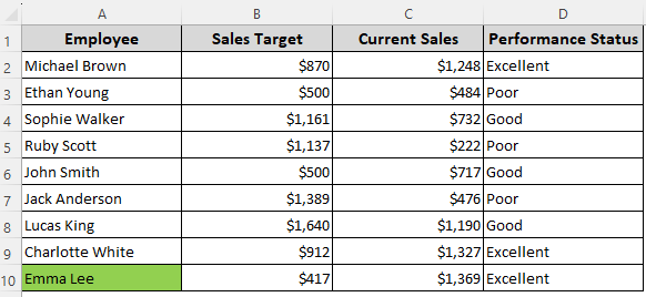
In our sample dataset, we have columns for employee names, sales targets, current sales, and performance status.
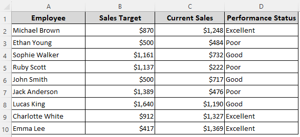
Here, we’ll look into the values of Column B and highlight the cells in Column A if the value in Column B is equal to, greater than, or less than $500.
➤ Select the cells you want to highlight based on another column. We selected the range A2:A10.
➤ Go to the Home tab and click the Conditional Formatting drop-down in the Styles group. From the menu, select New Rule.
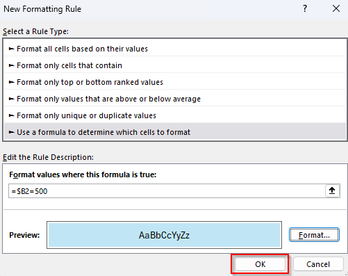
➤ As Excel opens the New Formatting Rule dialog box, select the Use a Formula to Determine Which Cells to Format option.
➤ In the Format Values Where This Formula Is True field, enter any of the following formulas:
Formula If Value Equals $500
=$B2=500
➤ $B2 is the first cell of the criteria range. Change it according to your dataset.
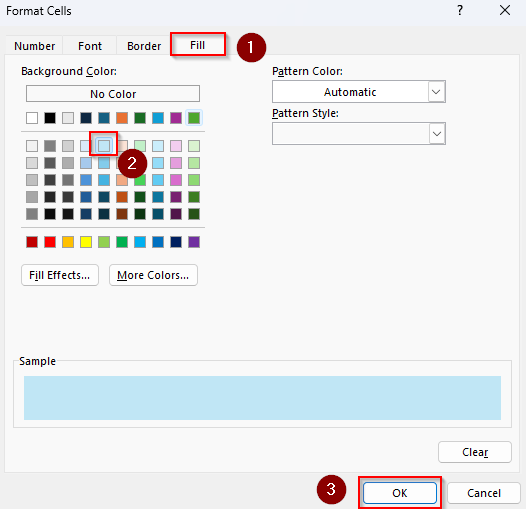
➤ Click on Format and choose your formatting (e.g., fill color, text color, font, etc.). Press Ok when you’re done.
➤ Close the New Formatting Rule dialog box by clicking Ok.
➤ Here’s the final result:
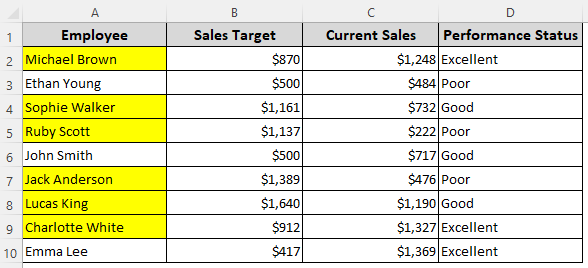
Formula If Value Is Greater Than $500
=$B2>500
➤ Replace $B2 with the first cell of the criteria range. Press Format to set formatting rules. Click Ok.
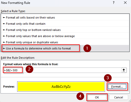
➤ Press Ok to close the dialog box and see the formatted data.
Formula If Value Is Less Than $500
=$B2<500
➤ Change $B2 as required and use the Format button to set formatting options. Press Ok and close the dialog box.
➤ Below is our final dataset:
Compare Values in Two Columns and Format Based on the Values
Instead of formatting based on a specific value, here we’ll compare the values in two columns and format one based on the values of another column.
For example, we’ll see if the values in Column B if the values in Column B are greater or less than the corresponding values in Column C. If yes, the formula will highlight the cells in Column B. Below are the steps:
➤ Select the range where you want to apply the formatting and click on the Home tab >> Conditional Formatting drop-down >> New Rule >> Use a Formula to Determine Which Cells to Format.
➤ Insert any of the following formulas in the Format Values Where This Formula Is True box:
Formula for Values Greater Than Column C
=$B2>$C2
➤ $B2 and $C2 are the first cells of columns we’re comparing. Change the values based on your dataset.
➤ Use the Format button to select formatting styles. Press Ok when you’re done.
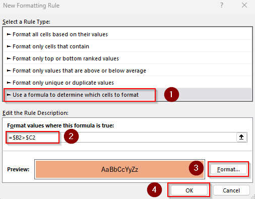
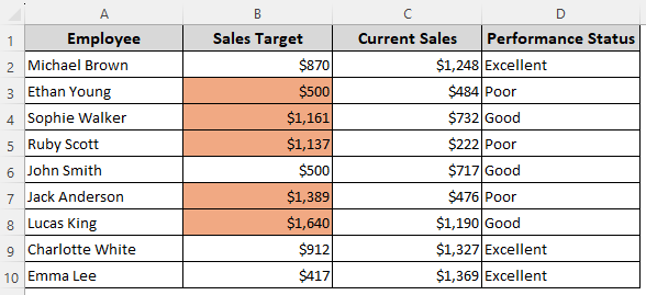
➤ Click Ok and check the final output.
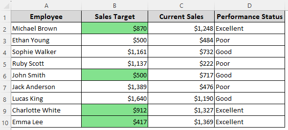
Formula for Values Less Than Column C
=$B2<$C2
➤ Replace $B2 and $C2 as needed. Press Format to set formatting options rules click Ok.
➤ Close the dialog box by pressing the Ok button. Here’s the final result:
Highlight One Column When Another Column Meets Single or Multiple Conditions
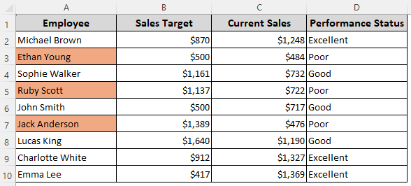
When applying formatting based on a single condition, we’ll check if Column D contains Poor and highlight the corresponding cell(s) in Column A accordingly. For multiple conditions, we’ll look for Poor in Column D and check if the values in Column C are less than $500.
Based on whether one or both conditions are met, we’ll highlight the cells in Column A. Let’s get to the steps:
➤ Select the range to apply conditional formatting rules and open the Home tab >> Conditional Formatting drop-down >> New Rule >> Use a Formula to Determine Which Cells to Format.
➤ In the formula box, type any of the following formulas:
Formula When a Single Condition Is Met
=$D2="Poor"
➤ Here, $D2 is the first cell of our criteria range. Change it to match your dataset.
➤ Apply formatting styles by pressing the Format button. Click Ok once done.
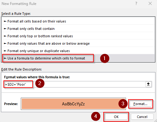
➤ Press Ok to apply the formatting and check the output:
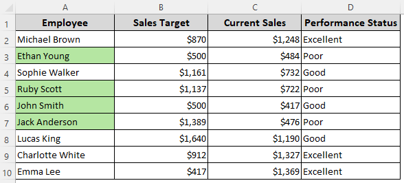
Formula When One of Multiple Conditions Is Met
=OR($D2="Poor",$C2<500)
➤ Replace $D2 and $C2 with the first cells of the criteria columns.
➤ Press Format, select the formatting options, and click Ok.
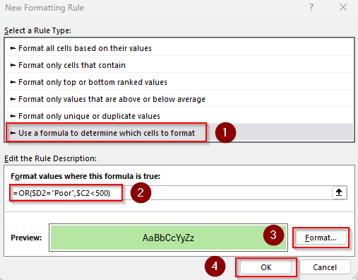
➤ Press Ok again to close the dialog box. Our final output is as follows:
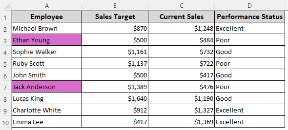
Formula When All Conditions Are Met
=AND($D2="Poor",$C2<500)
➤ Change $C2 and $D2 as required.
➤ Use the Format button to choose formatting styles and click Ok.
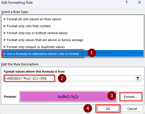
➤ Press Ok to see the final result.
Frequently Asked Questions
How to automatically apply conditional formatting rules for new entries based on the value in another column?
To automatically update the conditional formatting rules for new entries, you need to turn your dataset into a table. For this, select your data range and press Ctrl + T . When Excel prompts you, confirm the range and whether headers exist. Click Ok.
How to reference an entire column in an Excel formula?
You can reference an entire column in Excel by using the column letter(s) without row numbers. For example, here’s a typical formula:
=SUM(B:B)
This sums all values in Column B. While you use B:B in conditional formatting, it’s best to apply the rule to a range (e.g., B2:B100) instead of the full column, to avoid slowing down Excel.
How do I copy a conditional formatting rule to another cell?
For copying conditional formatting rules to a different cell, select a cell with the conditional formatting applied. Go to the Home tab >> Format Painter. Now, click on the cell(s) where you want to apply the same formatting.
Concluding Words
When formatting based on another column, always use an absolute column reference (e.g., $D in $D2) for the column you’re checking, and a relative row reference (e.g., 2 in $D2) for row-by-row evaluation.
You can view and edit all your rules by going to the Home tab >> Conditional Formatting >> Manage Rules. Here you can change their order (which rule is applied first), edit them, or delete them.