To highlight cells in a data range based on a date stored elsewhere in your sheet, you need to use a formula with an absolute reference (fixed with a dollar sign, $). Such formatting is used for tracking deadlines, monitoring project timelines, managing subscriptions, or highlighting upcoming events.
You can either use a single cell reference containing a date or compare dates in two different columns using the basic conditional formatting formulas and functions (greater than, less than, AND function, etc.).
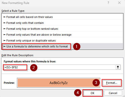
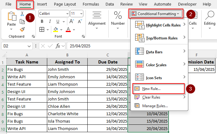
➤ Put the date in a cell (F2) and select the range you want to highlight (D2:D10). Go to the Home tab >> Conditional Formatting drop-down >> New Rule >> Use a Formula to Determine Which Cells to Format.
➤ To format the cells containing the dates after the date specified in F2 (overdue dates), enter this formula in the Format Values Where This Formula Is True box:
=D2>$F$2
➤ Here, D2 is the first cell of our data range and $F$2 contains the specified date. Change the values according to your dataset. Use the Format button to set formatting styles and press Ok.
In this article, we’ll cover how to apply conditional formatting rules to highlight dates that are on, before, after, or within X days of a date in another cell.
Highlight Dates That are On, Before, or After a Date in Another Cell
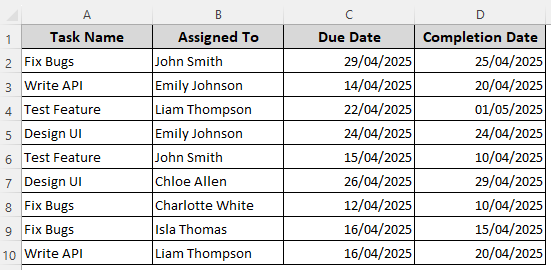
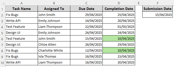
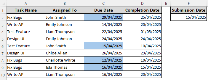
In our dataset, we have columns for project tasks, assignee names, deadlines, and completion dates. We’ll apply formatting rules to highlight overdue tasks, upcoming tasks, or completed ones based on the dates specified in a different cell(s).
First, let’s put the submission date in F2. To highlight the dates in Column D that are on, before, or after that submission date, follow the steps given below:
➤ Click and drag to select the column range to format. We’re selecting D2:D10. Now, go to the Home tab, click on the Conditional Formatting drop-down and choose New Rule.
➤ As Excel opens the New Formatting Rule dialog box, click on Use a Formula to Determine Which Cells to Format.
➤ In the blank field under the Format Values Where This Formula Is True option, insert any of the following formulas:
Highlight Dates Before the Date
=D2<$F$2
➤ Here, D2 is the first cell of our range. Change it according to your dataset.
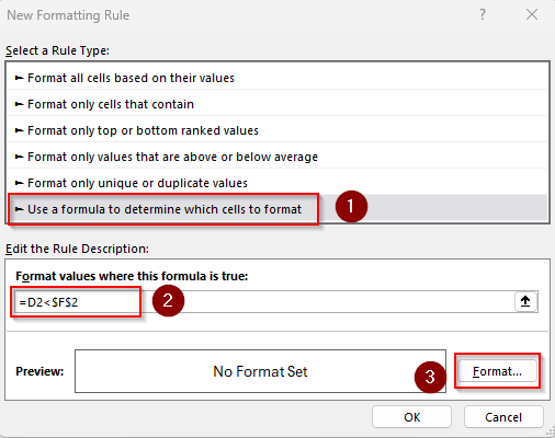
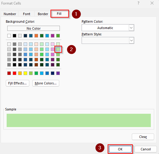
➤ Click on Format and use the Number, Font, Border, and Fill tabs to highlight the cells. Press Ok when you’re done.
➤ Close the New Formatting Rule dialog box by clicking the Ok button.
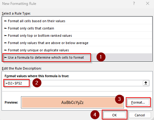
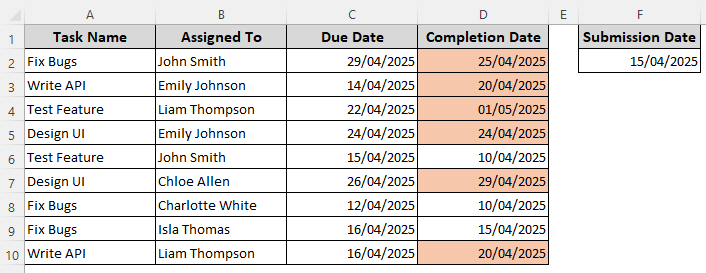
Highlight Dates After a Certain Date
=D2>$F$2
➤ Replace D2 with the first cell of your range. Use the Format button to apply highlighting options. Press Ok.
➤ Click Ok to close the dialog box and see the results.
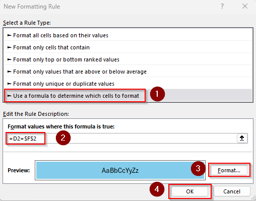
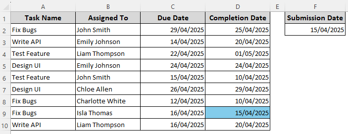
Highlight Dates Equal to a Certain Date
=D2=$F$2
➤ Change the values as needed and set formatting rules using the Format button. Press Ok.
➤ Click Ok and see the output:
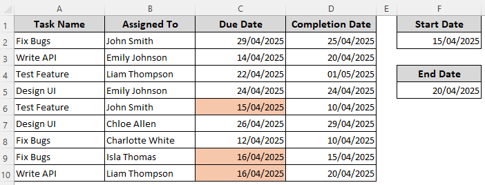
Format Dates That are Between Two Dates in Other Cells
In this method, we’ll enter two dates in two different cells and highlight the dates in Column B that are within those two dates. Let’s get to the steps:
➤ Enter the Start Date in F2 and the End Date in F5.
➤ Select the range of dates you want to highlight (we chose C2:C10) and open the Home tab >> Conditional Formatting drop-down >> New Rule >> Use a Formula to Determine Which Cells to Format.
➤ In the designated field for the formula, insert the following:
=AND(C2>=$F$2, C2<=$F$5)
➤ Replace the cell references as required, set formatting rules, and press Ok.
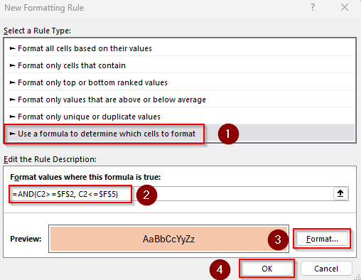
➤ Click Ok to close the window and the result should be as follows:
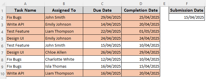
Highlight Entire Rows Based on a Date
Instead of formatting cells in a single column, we can highlight the entire row based on a date in another column. We’ll compare the date F2 against the dates in Column D to check if the dates in Column D are after the date in F2. Here’s how:
➤ Insert the date in F2 and select your entire dataset without the headers (A2:D10). We selected A2:D10. Now, click on the Home tab >> Conditional Formatting drop-down >> New Rule >> Use a Formula to Determine Which Cells to Format.
➤ In the formula box, enter the following formula to highlight rows where the date is after the one in F2:
=$D2>$F$2
➤ Replace $D2 with the first cell of the date range you’re comparing and change $F$2 to the cell containing the specified date.
➤ Click on Format to set formatting styles to highlight the cells. Once done, press Ok.
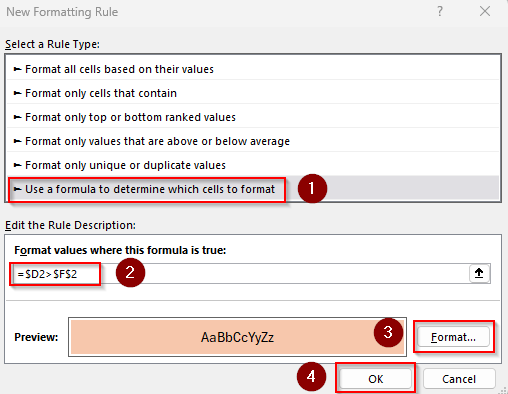
➤ Press Ok to close the window and see the highlighted rows.
Apply Conditional Formatting to Dates within X Days of a Date
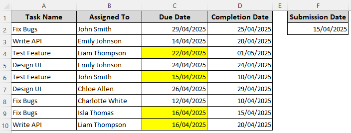
With the AND function, we can combine two or more conditions to highlight dates within X days of a date in another cell. Here, we’ll highlight dates in Column C that are within 7 days of the date in F2. Below are the steps:
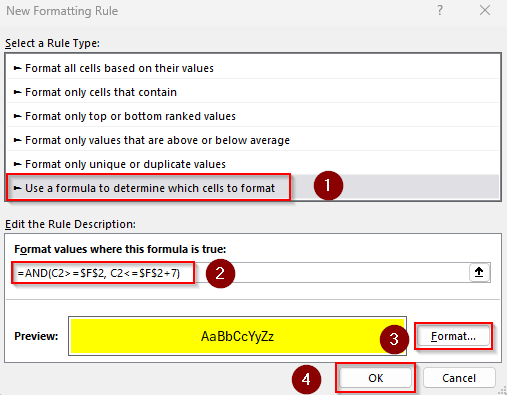
➤ Select your range (C2:C10) and go to the Home tab >> Conditional Formatting drop-down >> New Rule >> Use a Formula to Determine Which Cells to Format.
➤ In the blank field under the Format Values Where This Formula Is True box, enter the following formula:
=AND(C2>=$F$2, C2<=$F$2+7)
➤ C2 is the first cell of our range and $F$2 contains the date to compare against. Change the values as needed.
➤ Set formatting rules using the Format button and click Ok.
➤ Press Ok to close the dialog box and apply the highlighting rules.
Compare Dates in Different Columns
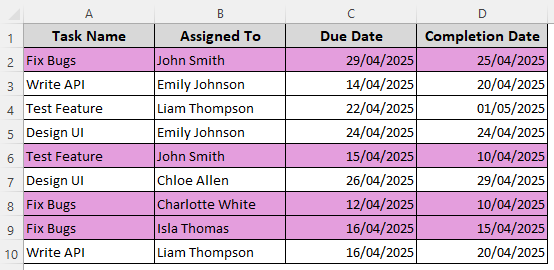
Our dataset has two columns for deadlines (Column C) and completion dates (Column D). To highlight overdue dates, we’ll highlight Column C dates that are after the dates in Column D. You can either highlight the entire row or just the cells in a single column. Here’s how:
Highlight the Entire Column
➤ Select your entire data range (A2:D10) and go to the Home tab >> Conditional Formatting drop-down >> New Rule >> Use a Formula to Determine Which Cells to Format.
➤ Insert the following formula in the formula box:
=$C2>$D2
➤ Change the references $C2 and $D2 with the first cells of the columns you’re comparing.
➤ Set formatting rules and press Ok.
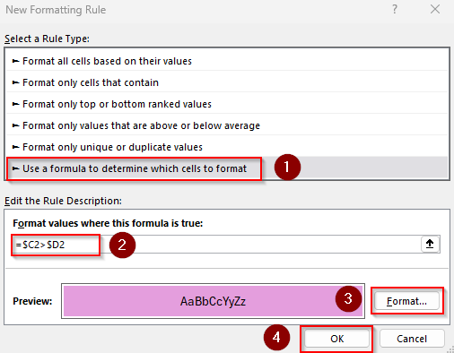
➤ Close the dialog box by clicking Ok and see the final output.
Highlight Cells in a Single Column
➤ Select the cells of the column (C2:C10) and go to the Home tab >> Conditional Formatting drop-down >> New Rule >> Use a Formula to Determine Which Cells to Format.
➤ In the formula field, enter the following formula:
=C2>D2
➤ Replace the cell references as needed and set formatting rules. Click Ok.
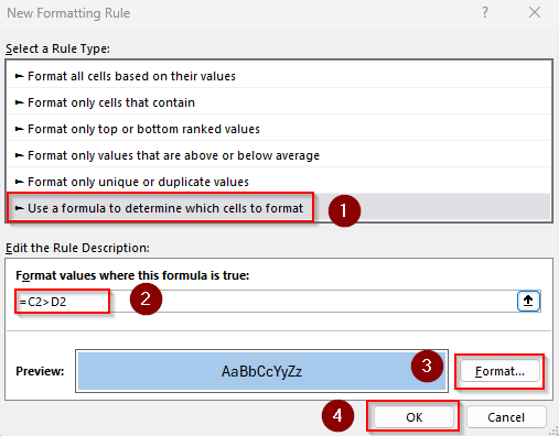
➤ Press Ok and the final result should be like this:
Highlighting Dates Based on Dates and Texts in Other Cells
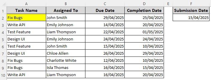
Use this method to highlight cells based on multiple conditions in different cells. We’ll highlight the cells in Column A if the employee is John Smith (in Column B), and the completion date (in Column D) is after the date in F2. Below are the steps:
➤ Select the range to apply formatting (A2:A10) and go to the Home tab >> Conditional Formatting drop-down >> New Rule >> Use a Formula to Determine Which Cells to Format.
➤ In the formula box, enter this formula:
=AND($B2="John Smith",$D2>$F$2)
➤ Here, $B2 is the first cell of the text condition column, $D2 is the first cell of the date condition column, and $F$2 contains the specified date. Replace the values according to your dataset.
➤ Apply the formatting rules using the Format option and press Ok once done.
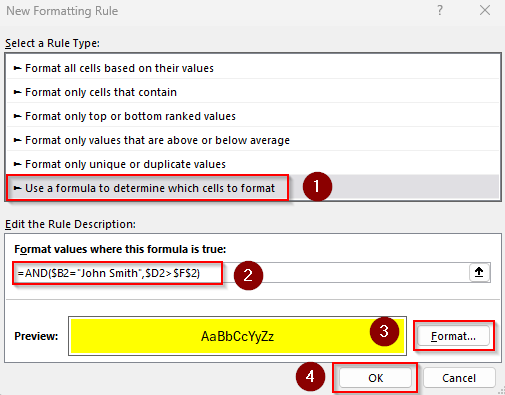
➤ Click Ok to check the final output:
Frequently Asked Questions
How do you conditionally format if the date is two days earlier than the due date in Excel?
Let’s say Column C contains actual dates and Column D has due dates. To highlight Column C when it is at least 2 days earlier than the due date in Column D, select the range (C2:C10) to highlight and Home tab >> Conditional Formatting drop-down >> New Rule >> Use a Formula to Determine Which Cells to Format. In the formula box, enter:
=$C2<=$D2-2
Set formatting rules and press Ok twice.
How to make Excel cells change color automatically based on expiry date?
First, enter the expiry dates in a column (Column E). To highlight expired items (expiry date is before today), select the range to format (E2:E10) and go to the Home tab >> Conditional Formatting drop-down >> New Rule >> Use a Formula to Determine Which Cells to Format.
Insert this formula in the designated box:
=E2<TODAY()
To highlight items still valid (expiry date after today), use this formula instead:
=E2>TODAY()
Set the formatting rules and click Ok twice.
How do I highlight the latest date in a column using conditional formatting?
If the dates are in Column C, select the range to highlight (C2:C10) and go to the Home tab >> Conditional Formatting drop-down >> New Rule >> Use a Formula to Determine Which Cells to Format. In the formula field, enter:
=C2=MAX($C$2:$C$10)
Select the formatting style and press Ok twice.
Concluding Words
When applying a conditional formatting rule, referencing a fixed control cell, lock the cell with $ if you’re referencing a fixed control cell. Lock the column with $ when you’re formatting based on a different column. You can also use the TODAY function to highlight cells based on the current date.