
Combining the IF statement with Conditional Formatting in Excel allows users to create dynamic rules that automatically highlight cells based on logical conditions. With Excel’s built-in tools and functions, we can easily highlight specific cells and make data easier to identify.
Follow the steps below to use IF statement with Conditional Formatting in Excel:
➤ In your dataset, head to the column where you want to apply conditional formatting and paste the following formula:|
=IF([Value1] >= [Value2], [ResultIfTrue], [ResultIfFalse])
➤ Replace “Value 1” with the cell reference of first value you want to test.
➤ Replace “Value 2” with the cell reference value you are comparing against
➤ Replace “ResultIfTrue” with the text to be displayed if the condition is true.
➤ Replace “ResultIfFalse” with the text to be displayed if the condition is false.
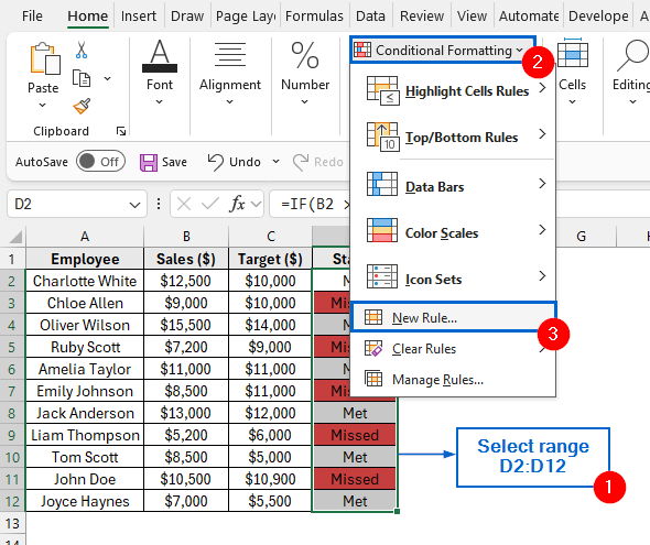
➤ Then, head to Conditional Formatting >> New Rule.
➤ Select Use a formula to determine which cells to format option and under Format values where this formula is true field, enter the following formula:
=$B2 <$C2
➤ Replace $B2 with the cell reference of the first value you want to compare.
➤ Replace $C2 with the cell reference of the second value you want to compare.
➤ Next, choose a fill colour, and repeat the process to create another rule for values greater than or equal to your criteria.
In this article, we will learn three effective methods of using IF statement in Excel Conditional Formatting.
Using IF Statement with a Helper Column to Highlight Cells
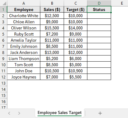
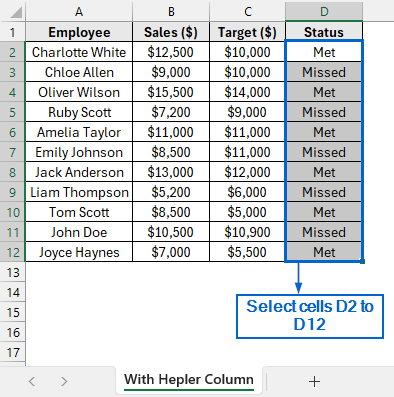
In the sample dataset, we have a worksheet called “Employee Sales Target” containing information about Employee names, Sales, Target and an empty Status column that will act as a helper column.
By combining the IF statement with Conditional Formatting, we will display “Met” or “Missed” in column D and highlight the cells in green or red based on whether employees meet their sales targets. The updated dataset will be stored in a separate “With Helper Column” worksheet.
The IF statement in Excel is a logical function that returns one value if a condition is true and another value if the condition is false. Follow the steps below to apply the IF statement with Conditional Formatting to your dataset.
Step 1: Apply the IF Statement
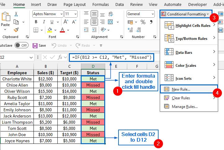
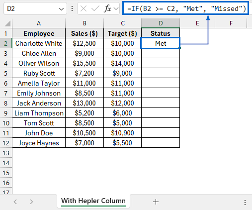
➤ Head to the With Helper Column worksheet, select cell D2, and paste the following formula:
=IF(B2 >= C2, "Met", "Missed")
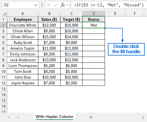
➤ Now, select cell D2 again and double-click the fill handle to apply the formula across the entire column.
Step 2: Apply Conditional Formatting to Define a Target Value
➤ Next, select cells D2 to D12.
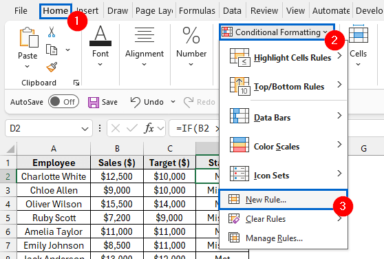
➤ From the main menu, head to Conditional Formatting >> New Rule.
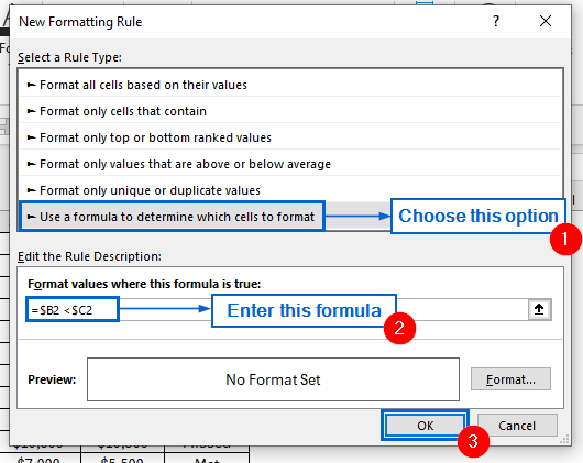
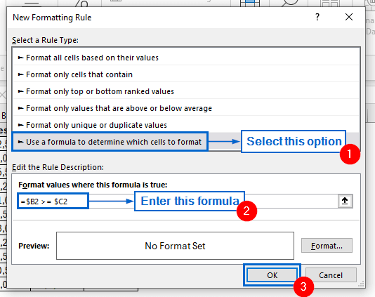
➤ In the New Formatting Rule dialogue box, choose Use a formula to determine which cells to format option. Next, type the formula into the Format values where this formula is true box and click Format.
=$B2 <$C2
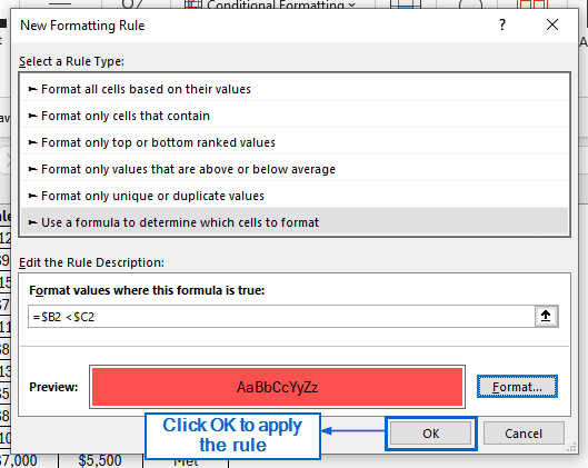
➤ Next, go to the Fill tab from the Format Cells dialogue box, choose a red colour, and click OK.

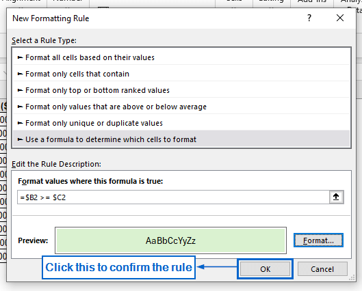
➤ Finally, in the New Formatting Rule dialogue box, click OK to apply the formatting rule.
Step 3: Apply Conditional Formatting for Not Meeting the Defined Target
➤ Head to the dataset again, select cells D2:D12, then head to Conditional Formatting >> New Rule.
➤ From the New Formatting Rule dialogue box, choose the option Use a formula to determine which cells to format. Next, enter the formula into the Format values where this formula is true box and click Format.
=$B2 >= $C2
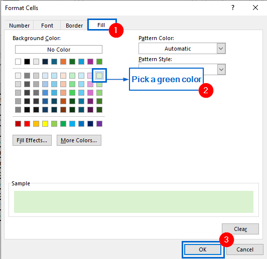
➤ Go to the Format Cells dialogue box, from the Fill tab pick a green fill colour, and click OK.

Step 4: Confirm Rules and Display the Results
➤ Finally, click OK in the New Formatting Rule dialogue box to apply the rules to your dataset.
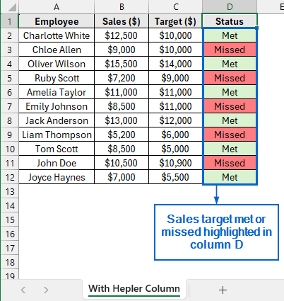
➤ Column D should now display whether the sales target is met or missed, with the cells highlighted in green or red accordingly.
Directly Use IF Statement in Conditional Formatting Without Helper Column
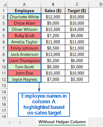
Unlike the previous method, this approach does not require a helper column to use the IF statement. Using the same dataset, we will now apply IF statement directly within Conditional Formatting to highlight the employee names in column A, marking them in green or red depending on whether they meet the sales target. We will display the updated dataset in a separate “Without Helper Column” dataset.
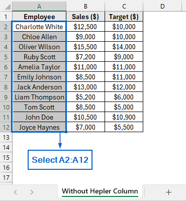
➤ Head to the Without Helper Column worksheet and select cells A2:A12.
➤ From the main menu, select Conditional Formatting >> New Rule.
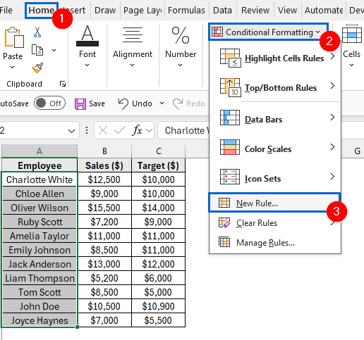
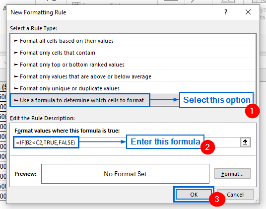
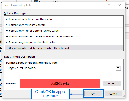
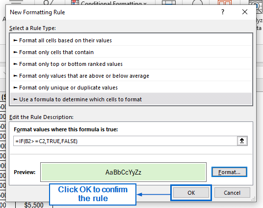
➤ In the New Formatting Rule window, choose Use a formula to determine which cells to format option. Enter the formula below into the input box, then click Format.
=IF(B2<C2,TRUE,FALSE)
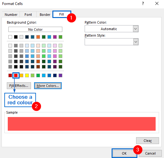
➤ Next, open the Fill tab from Format Cells dialogue box, choose a red fill colour and press OK.
➤ Click OK again from the New Formatting Rule dialogue box to apply the formatting rule.
➤ Head to the dataset again, select range A2:A12 and head to Conditional Formatting >> New Rule.
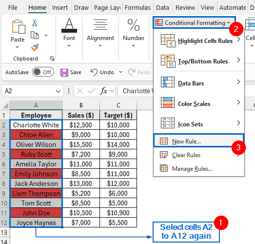
➤ Select Use a formula to determine which cells to format option, enter the following formula in the box, and click Format.
=IF(B2>=C2,TRUE,FALSE)
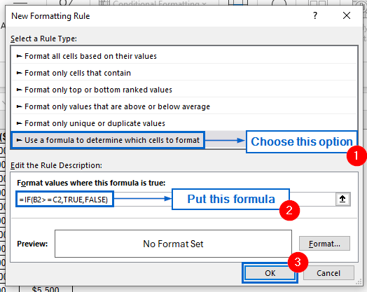
➤ Head to the Fill tab again, choose a green colour, then press OK to confirm selection.
➤ Finally, click on OK from the New Formatting Rule dialogue box to apply the rules.
➤ Employee names in Column A of the dataset should now be highlighted in red or green, depending on meeting sales targets.
Automatically Use IF Statement in Conditional Formatting with VBA Editor
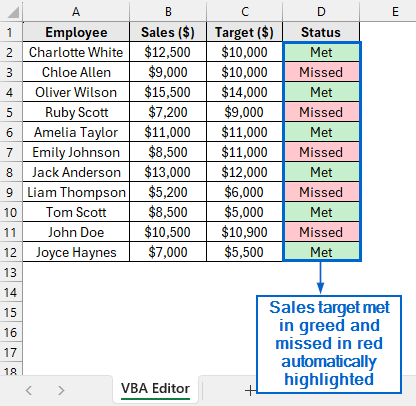
The VBA Editor in Excel is a powerful tool which allows users to create custom macros to automate repetitive processes and save time. Working with the same dataset again, we will now display whether the sales target is “Met” or “Missed” in column D and highlight the cells in green or red. The updated dataset will be displayed in a separate “VBA Editor” worksheet.
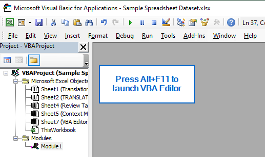
➤ Head to the VBA Editor worksheet and Alt + F11 to launch the VBA Editor window.
➤ Next, from the VBA window, go to Insert >> Module and paste the following script.
Sub ApplyIFWithHelperColumn()
    Dim ws As Worksheet, lastRow As Long, rng As Range
    Set ws = ActiveSheet
    lastRow = ws.Cells(ws.Rows.Count, "A").End(xlUp).Row
    ws.Range("D2:D" & lastRow).Formula = "=IF(B2>=C2,""Met"",""Missed"")"
    Set rng = ws.Range("D2:D" & lastRow)
    rng.FormatConditions.Delete
    rng.FormatConditions.Add(Type:=xlExpression, Formula1:="=$D2=""Met""").Interior.Color = RGB(198, 239, 206)
    rng.FormatConditions.Add(Type:=xlExpression, Formula1:="=$D2=""Missed""").Interior.Color = RGB(255, 199, 206)
End Sub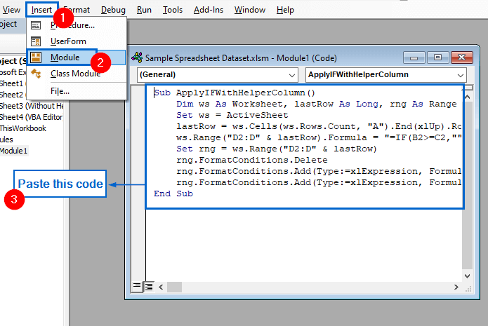
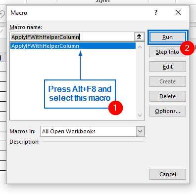
➤ Now, exit the VBA window, press Alt + F8 to launch the Macros dialogue box, choose the ApplyIFWithHelperColumn macro, and click Run.
➤ Column D should now display sales targets met in green and missed in red.
Frequently Asked Questions
Which Method Works Best for Large Datasets?
For large datasets, using IF statement directly inside Conditional Formatting and VBA Editor would be the best since both methods can quickly process data and reduce unnecessary clutter.
What Happens If My Dataset Contains Blank Cells?
If your dataset contains blank cells, both the Conditional Formatting with IF statement methods and the VBA Editor will automatically skip them. This ensures that only valid results are highlighted, improving overall data readability.
Concluding Words
Knowing how to use IF statement with Conditional Formatting in Excel is essential for creating dynamic rules and highlighting important data points.
In this article, we have discussed three effective methods of using IF statements in Excel Conditional Formatting, including using IF statements with helper column, without helper column and VBA Editor. Feel free to try all three methods and choose one that best suits your needs.