Pivot Tables are used for summarizing and analyzing large datasets in Excel. To focus analysis on specific subsets of data, filtering is important. While manually checking boxes in the filter dropdown works, Label Filters, Value Filters, Slicers, and Timelines offer dynamic ways to analyze your data based on text, numbers, or dates. In this article, we will guide you through several effective methods for filtering Pivot Tables based on cell value.
To filter Pivot Table based on cell value, here is one simple solution by using the search box.
➤ Press the dropdown icon from the Product label.
➤ In the search box, write down the text you want to search for, like “Oneplus”.
➤ Click OK, and the Pivot Table will display only the products containing “Oneplus”, confirming proper filtering based on cell value.
Using Filter Dropdown in Column Header
The quickest way to filter a Pivot Table for specific text is by using the search box directly within the filter dropdown.
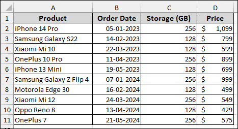
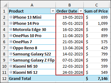
Imagine a sample dataset containing Product, Order Date, Storage (GB), and Price. Now, we will create a Pivot Table and then use filtering based on the cell values.
First, let’s create the Pivot Table.
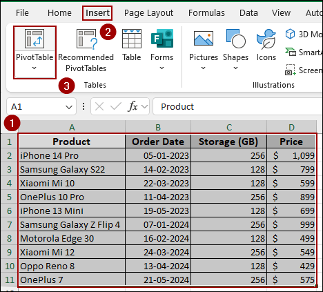
➤ Select your dataset.
➤ Go to the Insert tab and click PivotTable.
➤ In the dialog box, select New Worksheet and click OK.

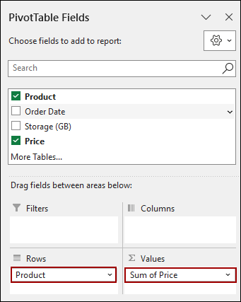
➤ In the PivotTable Fields pane, drag the Product field into the Rows area.
➤ Drag the Price field into the Values area. Excel automatically names this field Sum of Price.
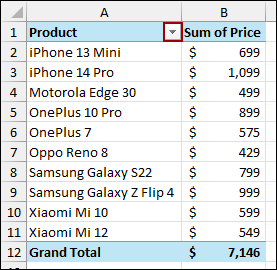
The resulting Pivot Table shows the total sum of prices for each product.
➤ Click the filter dropdown arrow next to the Product label.
➤ In the dropdown menu, type the text you want to search for, like “Oneplus“.
➤ Click OK.
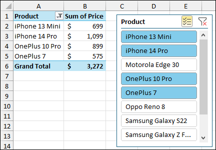
Excel automatically shows only the items that match your search. Ensure the desired items are check-marked.

The Pivot Table now displays only the products containing “Oneplus“.

Using Label Filters to Filter Text Values
Label Filters enable you to filter the row labels (the product names in our example) using specific text conditions, such as “begins with” or “contains”.
Filtering Values With Exact Text
To show a Pivot Table item that exactly matches a text string.
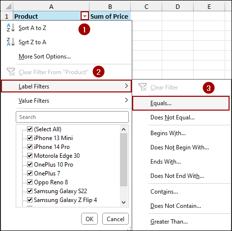
➤ Click the filter dropdown arrow next to Product.
➤ Hover over Label Filters and select Equals.
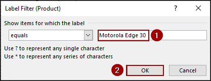
➤ In the Label Filter dialog box, type the exact product name, such as “Motorola Edge 30“.
➤ Click OK.
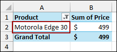
The Pivot Table is filtered to show only the “Motorola Edge 30“.
Filtering Based on Words Starting with Specific Text
To filter products that start with a common word.
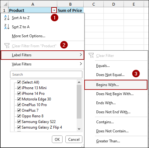
➤ Open the dropdown, hover over Label Filters, and select Begins With.
➤ In the dialog box, type “iPhone“.
➤ Click OK.
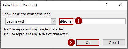
This displays only the iPhone products.
Filtering Values That End with a Specific Text
You can filter for a specific ending, which is helpful for model names.
➤ Open the dropdown, hover over Label Filters, and select Ends With.
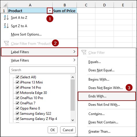
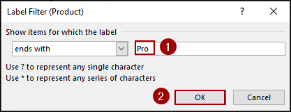
➤ In the dialog box, type “Pro“.
➤ Click OK.
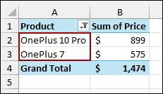
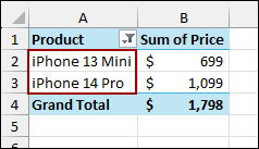
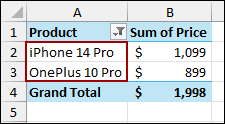
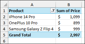
The Pivot Table is filtered to show products ending in “Pro“, such as “iPhone 14 Pro” and “OnePlus 10 Pro“.
Filtering Based on Partial Match
Use the “Contains” filter option to find products where the text appears anywhere in the name.
➤ Open the dropdown, hover over Label Filters, and select Contains.
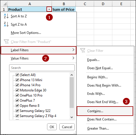
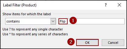
➤ In the dialog box, type “Flip“.
➤ Click OK.
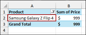
The result shows the “Samsung Galaxy Z Flip 4“.
Utilizing Value Filters to Filter Numeric Values
Value Filters analyze the summarized numerical data (e.g., Sum of Price), not the row labels. This allows you to identify products based on their total prices.
Exact Numeric Value
To filter for a specific summed value.
➤ Click the dropdown, hover over Value Filters, and select Equals.
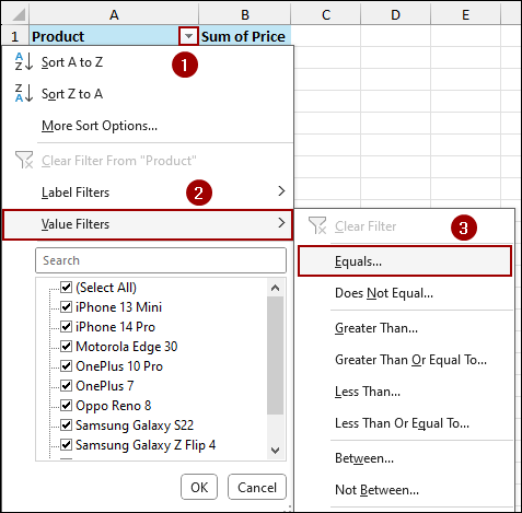
➤ In the dialog box, ensure Sum of Price is selected, then enter the price, such as 499.
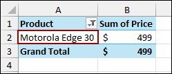
➤ Click OK.

The result shows the single product whose price equals $499.
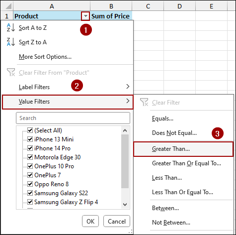
Greater Than Specific Value
To see only high-value items.
➤ Open the dropdown, hover over Value Filters, and select Greater Than.
➤ In the dialog box, enter a minimum value, like 799.
➤ Click OK.
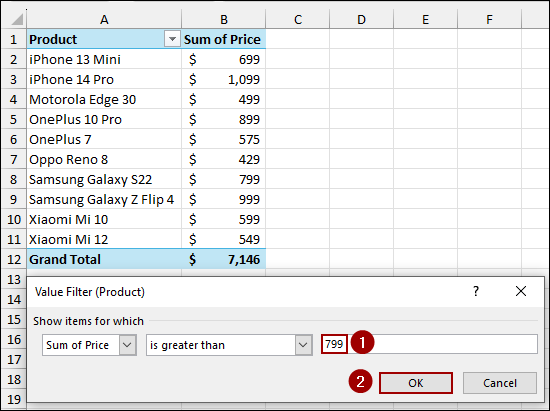
The Pivot Table now lists all products with a sum of price greater than $799.
Lower Than Specific Value
To analyze lower-value items.
➤ Open the dropdown, hover over Value Filters, and select Less Than.
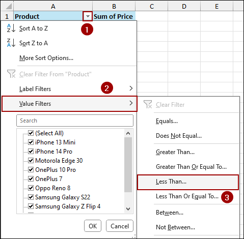
➤ In the dialog box, enter a maximum value, such as 599.
➤ Click OK.
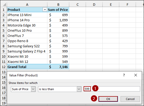
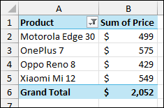
This filters the products to those with a sum of price less than $599.
Between Two Values
To specify a value range.
➤ Open the dropdown, hover over Value Filters, and select Between.
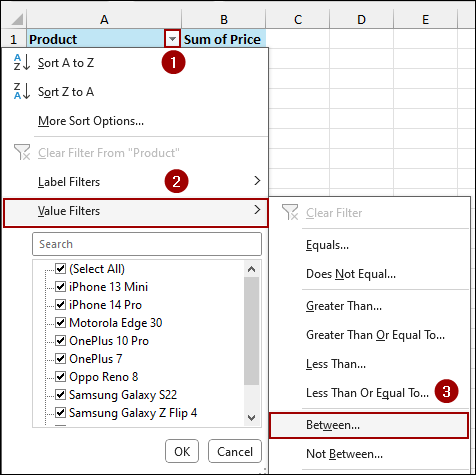
➤ Enter the lower value, 599, and the upper value, 900.
➤ Click OK.
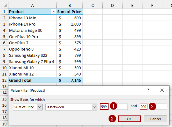
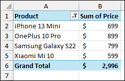
The table is filtered to display items whose prices fall between $599 and $900.
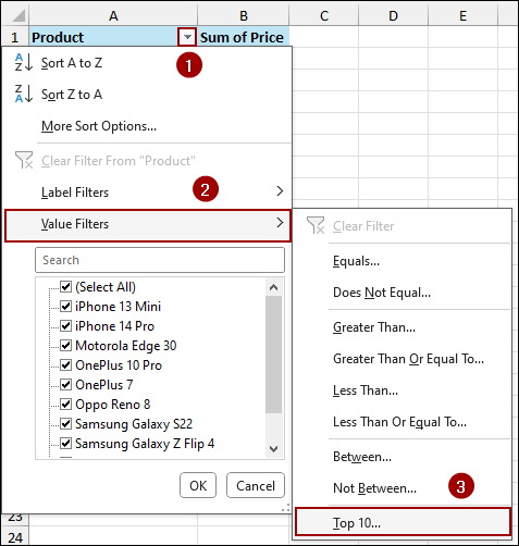
Top 5 Values
To quickly identify the best-selling or highest-priced items.
➤ Open the dropdown, hover over Value Filters, and select Top 10.
In the Top 10 Filter dialog box.
➤ Change Show to Top and the number field from 10 to 5.
Ensure the filters by Items by Sum of Price.
➤ Click OK.
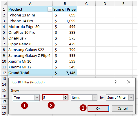
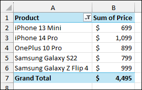
The Pivot Table is reduced to the Top 5 most expensive products.
Filter Pivot Table Data Using Slicer
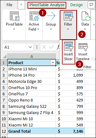
Slicers are one of the best tools that provide visual buttons for filtering Pivot Table data. Here, we will use Slicer to filter products based on cell value in the Pivot Table.
➤ Select any cell within your Pivot Table.
➤ Go to the PivotTable Analyze tab.
➤ In the Filter group, click Insert Slicer.
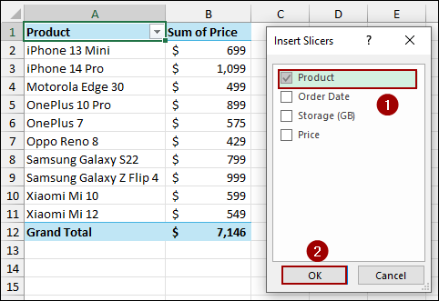
➤ In the Insert Slicers dialog box, check the box next to the field you want to filter by, in this case, Product.
➤ Click OK.
A Slicer pane will appear next to your Pivot Table. You can click on any product button to filter the Pivot Table instantly. To select multiple items, hold down the Ctrl key while clicking the buttons.
Inserting Timeline to Filter Dates
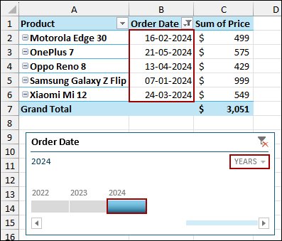
If your Pivot Table includes a date field, the Timeline feature is the best tool for filtering dates. Here, we will use the Insert Timeline feature to filter dates based on cell values in the Pivot Table.
➤ Drag the Order Date field into the Rows area alongside the Product field.
➤ Select any cell within the Pivot Table.
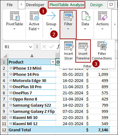
➤ Go to the PivotTable Analyze tab.
➤ In the Filter group, click Insert Timeline.
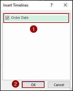
➤ In the Insert Timelines dialog, checkmark the box for the date field, Order Date.
➤ Click OK.
A Timeline pane will appear. You can use the timescale dropdown (set to Years, Quarters, or Months) and click or drag the selector to filter your Pivot Table data for that period.
Here, we have selected the bar for 2024 and filtered the Pivot Table to only show transactions that occurred in that year.
Frequently Asked Questions
Can I filter a Pivot Table using a cell value outside the table?
No. Pivot Table filters, Value Filters, and Label Filters are built into the structure of the Pivot Table fields. To filter dynamically based on a value in a cell outside the Pivot Table, you need to use a VBA macro or the Report Filter feature combined with the “Show Report Filter Pages” option.
Why is the Value Filter option greyed out?
Value Filters only appear for fields placed in the Rows or Columns areas that have a summarized numeric value (like Sum of Price) in the Values area. If your Pivot Table only contains text fields or the selected field is already in the Filters area, the Value Filter option will be disabled.
Can I apply multiple Slicers to one Pivot Table?
Yes. You can insert multiple Slicers for different fields and connect them all to the same Pivot Table. This allows you to apply layered, interactive filters simultaneously.
Concluding Words
Above, we have explored the most effective methods to filter data in an Excel Pivot Table based on cell value. From using the quick Search Box and precise Label/Value Filters to applying the Slicers and Timelines, you can easily filter data, setting desired criteria. If you have any further questions, please don’t hesitate to share them in the comments section below.