
Filtering by multiple colors in Excel means displaying rows that match more than one cell color simultaneously. For example, both “Yellow” (In Progress) and “Green” (Completed) statuses. Since Excel’s built-in filter supports only one color at a time, we use helper columns or VBA functions to assign color codes, allowing flexible multi-color filtering. This feature is good for project managers, data analysts, and sales teams who rely on visual indicators in large datasets.
To filter by multiple colors in Excel, follow these steps:
➤ Assign color codes to each colored cell using a VBA function.
➤ Apply the FindColor formula to extract numeric color codes in a helper column.
➤ Use the Filter feature on that column to display multiple color-coded results.
In this article will describe two ways to filter by multiple colors in Excel using Color Codes and VBA Macro.
Using Color Code to Filter by Multiple Colors in Excel
Numeric color codes in a helper column are used to represent each cell color. By filtering these numeric values, we can view multiple color categories at once. This is good for sales performance sheets, task tracking lists, or project dashboards where colors indicate different progress or status levels.
We have a dataset that contains sales performance data of a company. We will use color code methods to represent the performance of specific sales regions.
Steps:
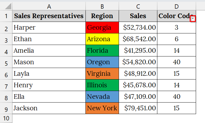
➤ Open your Excel file that contains your data. Here, we have taken a color-based table that contains Sales Representatives in Column A, Region in Column B, and Sales in Column C.
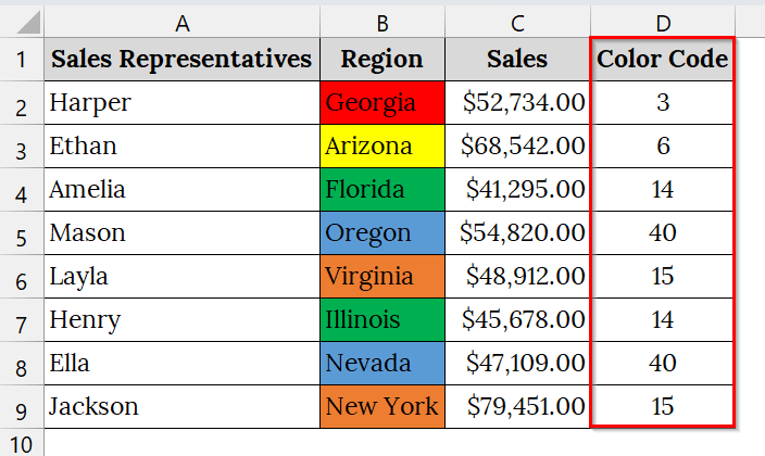
➤ Add a helper column and rename it as Color Code. Enter numeric Color Codes in Column D according to your color meanings:
➥ Red = 3
➥ Yellow = 6
➥ Green = 14
➥ Blue = 40
➥ Orange = 15
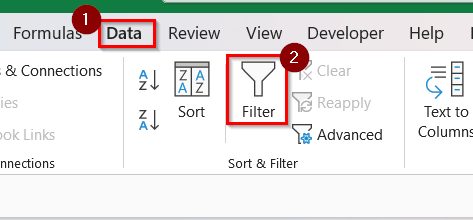
➤ Then, go to the Data tab → Sort & Filter group → click Filter.
➤ This will add drop-down arrows to the column headers.
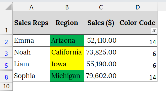
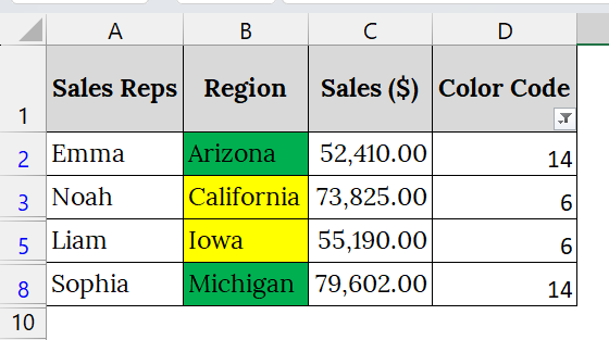
➤ Click the drop-down arrow in the Color Code column. From the filter list, check the boxes for 14 (Green) and 40 (Blue). Click OK.
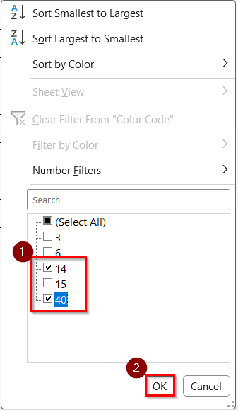
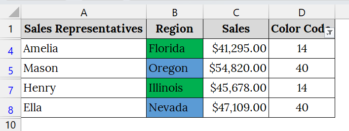
➤ Excel will now show only the rows with Blue (14) and Green (40) color codes.
Applying a VBA Macro to Filter by Multiple Colors in Excel
We usually extract and filter cell colors using a VBA function that returns the color code of each cell. This is good when our Excel sheet uses background colors to represent performance levels, progress stages, or categories, and we need to filter by multiple colors simultaneously.
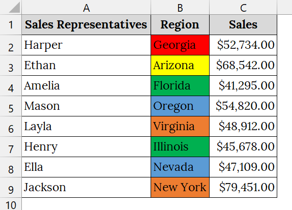
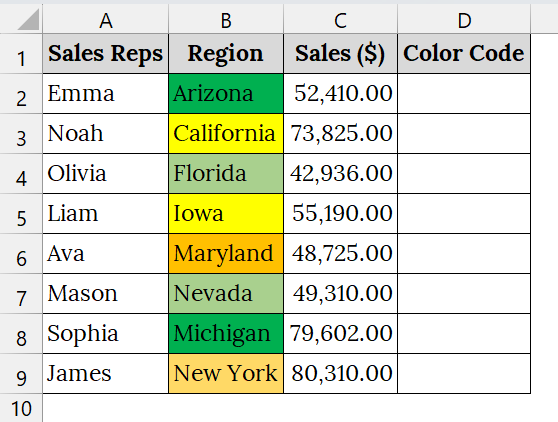
We have a dataset of BlueWave Electronics that contains color-coded regions based on sales performance: Here, the color refers to Red (3) = Low Sales, Yellow (6) = Average Sales, Green (14) = Good Sales, Orange (15) = Above Average, Blue (40) = Excellent Sales. We will filter by multiple colors using the VBA Macro to review both “Good” and “Average” performance together.
Steps:
➤ Open your Excel file that uses background color to represent your information. For example, we have taken a color-based table that contains Sales Representatives in Column A, Region in Column B, and Sales in Column C, and a helper Column (Color Code) in Column D.
➤ Press the keyboard shortcut Alt + F11 to open the Microsoft Visual Basic for Applications window directly.
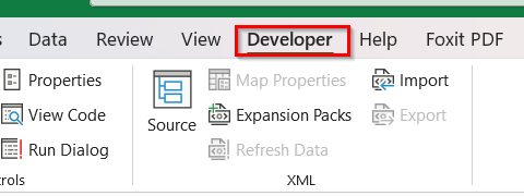
➤ Or, go to the Developer tab on the Excel ribbon.
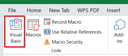
➤ Select Visual Basic.
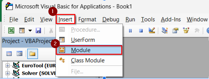
➤ In the Microsoft Visual Basic for Applications window, click Insert from the top menu and choose Module.
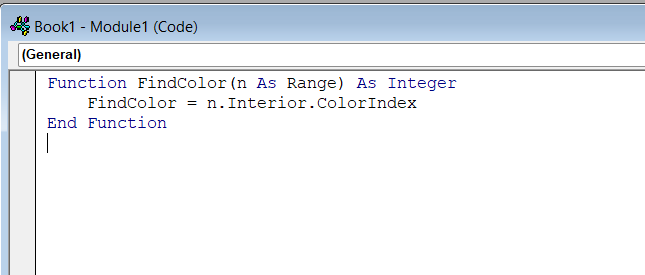
➤ In the Module window, paste the following code:
Function FindColor(n As Range) As Integer
    FindColor = n.Interior.ColorIndex
End Function
This code creates a custom function named FindColor, which returns the color index of the selected cell.
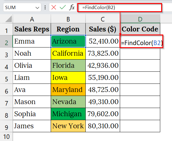
➤ Close the VBA window and return to your Excel worksheet. In cell D2, enter the formula:
=FindColor(B2)
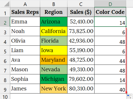
➤ Press Enter, then drag the Fill Handle down the column to copy the formula for other rows. You will now see numeric color codes appear beside each colored cell.
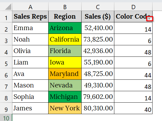
➤ Then, go to the Data tab → Sort & Filter group → click Filter.

➤ Click the filter dropdown on the Color Code column.
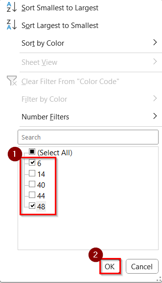
➤ From the filter list, check the boxes for Green (14) to filter good sales and Yellow (6) to filter average sales.
➤ Click OK.
➤ Excel now displays only the rows that match the selected color codes (multiple colors filtered at once).
Note:
➥ The FindColor function only works for cell background colors, not conditional formatting colors.
➥ Always save your workbook as .xlsm (Macro-Enabled Workbook) to retain the VBA function.
Frequently Asked Questions
Can I filter multiple colors without VBA?
Yes, by assigning manual color codes in a helper column and filtering those numeric values, you can filter multiple colors even without using VBA.
Does this method work with conditional formatting?
No, VBA’s FindColor function identifies static background colors only. Conditional formatting colors require different VBA approaches.
What are the most common color codes in Excel?
Some default color indexes include Red = 3, Yellow = 6, Green = 14, and Blue = 40.
Why should I use color codes instead of just visual filters?
Color codes give you flexibility. You can filter, sort, or combine multiple colors efficiently, especially in large datasets.
Concluding Words
Filtering by multiple colors in Excel is quite easy using the Color Code and VBA Macro Method. These approaches increase visibility, improve data organization, and simplify color-based reporting in Excel. Also, we have uploaded all the datasets used in this article, so that you can download and use them for practice.