Creating a professional and dynamic report card in Excel is essential for managing student performance data. A well-designed report card displays a student’s information, marks, grades, and overall percentage using powerful lookup functions. This not only saves time but also minimizes data entry errors. In this article, we will guide you through a step-by-step process of creating a professional report card from scratch.
To make a report card in Excel, here is one simple solution by using the combination of VLOOKUP and MATCH functions.
➤ Prepare a dataset with all students and mark information.
➤ Design the report card structure using shapes and formatting.
➤ Use the Data Validation feature to create a dynamic drop-down list for selecting a Student ID.
➤ Apply VLOOKUP and MATCH formulas to get student details and subject marks automatically.
➤ Calculate the overall grade and percentage using SUM and nested IF functions to make the report card in Excel.
Steps to Make a Report Card in Excel
Here, we will use a step-by-step process to make a report card in Excel. We have broken down the process into four simple steps: preparing the dataset, designing the report card layout, implementing dynamic data retrieval, and calculating final results.
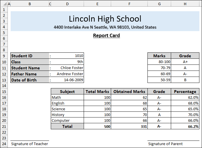
Step 1: Preparing the Dataset
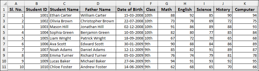
For creating a dynamic report card for students, we will make structured data first. This data will serve as the source from which all student-specific information will be pulled.
➤ Input your raw data, including columns for Sl. No., Student ID, Student Name, Father Name, Date of Birth, and marks for all subjects: Math, English, Science, History, and Computer.
This organized data table is crucial, as the Student ID column will act as the unique identifier for the lookup functions.
Step 2: Designing the Report Card Layout
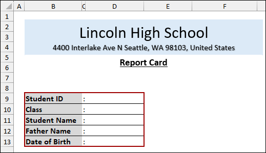
A professional appearance is essential for a report card. We will start by preparing the ‘Report’ sheet and adding basic elements.
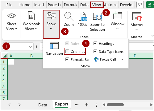
To make the report card look more like a document, we will remove the default gridlines.
➤ Select the new sheet and rename it to ‘Report’.
➤ Go to the View tab on the ribbon.
➤ In the Show group, uncheck the Gridlines option.
We will use shapes to create a header for the school and the report card title.
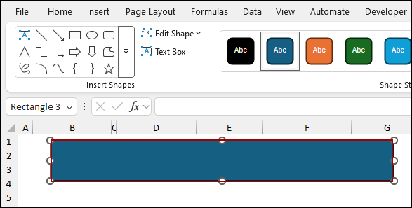
➤ Go to the Insert tab, click Illustrations, then select Shapes, and choose the Rectangle shape.
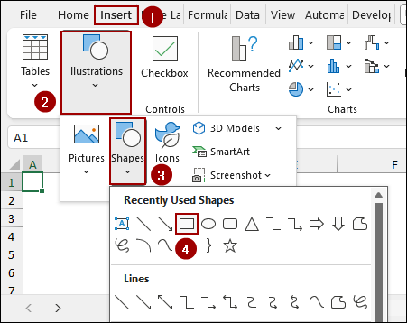
➤ Draw a large rectangle across the top of the sheet.
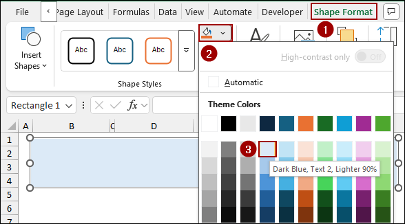
➤ With the shape selected, go to the Shape Format tab.
➤ Use the Shape Fill option to choose a light color (e.g., Dark Blue, Text 2, Lighter 90%).
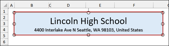
➤ Add text to the shape by typing the school’s name and address.
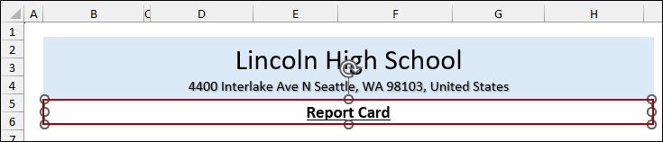
➤ Insert a Text Box shape and type “Report Card” and format it to be centered and underlined.
Next, we will set up the main sections for student details and the grading table.
➤ In the main body of the report, create a formatted table layout for Student ID, Class, Student Name, Father Name, and Date of Birth.
➤ Apply borders for a clean look.
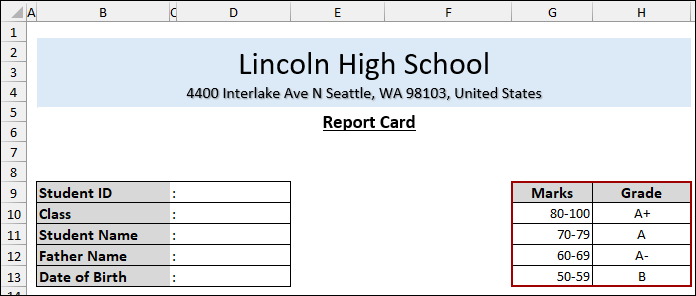
To the right, we will create a static table for the grading key.
➤ Create a small table displaying the Marks range and the corresponding Grade (e.g., 80-100 = A+, 70-79 = A, etc.).
Step 3: Implementing Dynamic Data Retrieval
This is the core dynamic part of the report card. We will use Data Validation to easily switch between students and then use VLOOKUP and MATCH to pull the correct data.
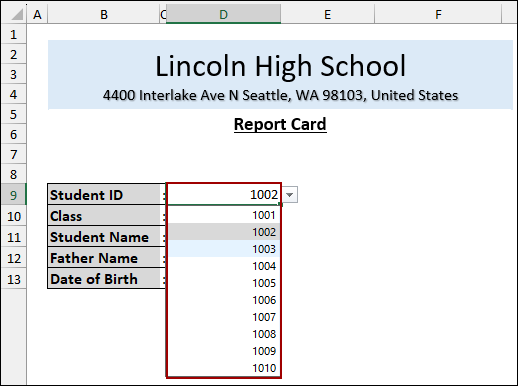
Instead of manually typing the ID, a drop-down list is more user-friendly.
➤ Select the cell where the Student ID will be entered (e.g., D9).
➤ Go to the Data tab, click Data Tools, and select Data Validation.
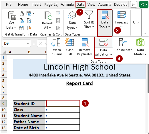
➤ In the Settings tab, choose List from the Allow dropdown.
➤ In the Source box, enter the range of Student IDs from your ‘Data’ sheet.
➤ Click OK.
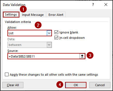
A dropdown arrow now appears in the cell, allowing you to select any Student ID from your list.
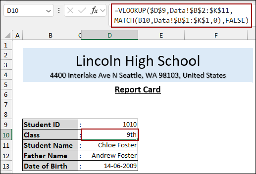
Now, we will use a combined VLOOKUP and MATCH functions to pull the student’s Class, Student Name, Father Name, and Date of Birth based on the selected Student ID.
➤ In the cell for Class (e.g., D10), enter the following formula, press ENTER, and drag down to fill.
=VLOOKUP($D$9, Data!$B$2:$K$11, MATCH(B10, Data!$B$1:$K$1, 0), FALSE)
➥ Data!$B$2:$K$11: The table array (the entire data table on the ‘Data’ sheet).
➥ MATCH(B10, Data!$B$1:$K$1, 0): This finds the column number for ‘Class’ dynamically by matching the text in cell B10 (which is “Class”) against the header row of the data table.
➥ FALSE: Ensures an exact match is found.
➤ Now, set up the subject breakdown table with columns for Subject, Total Marks, Obtained Marks, Grade, and Percentage.
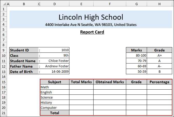
➤ Enter the Total Marks (e.g., 100) for each subject.
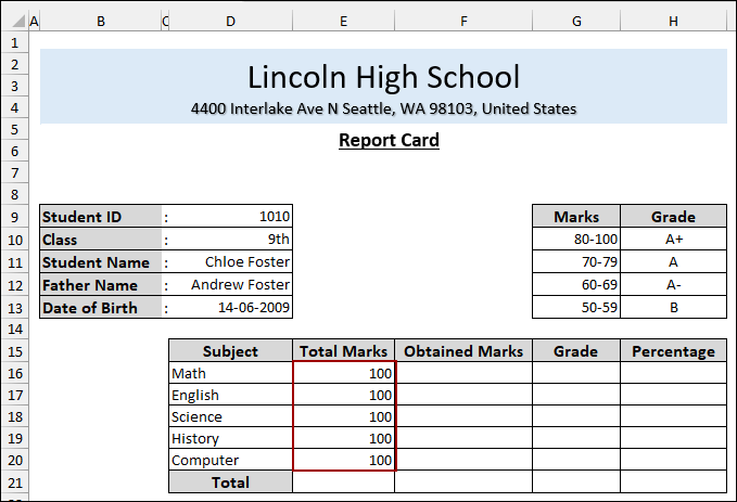
We will use the same dynamic formula to pull the marks for each subject.
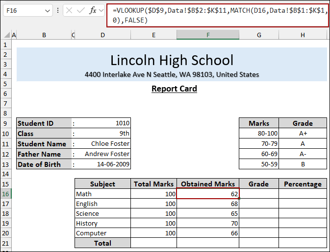
➤ In the cell for the first subject’s Obtained Marks (e.g., F16 for Math), enter the formula, press ENTER, and drag down the Fill Handle.
=VLOOKUP($D$9, Data!$B$2:$K$11, MATCH(D16, Data!$B$1:$K$1, 0), FALSE)
➥ Data!$B$2:$K$11: The table array.
➥ MATCH(D16, Data!$B$1:$K$1, 0): This finds the column number for ‘Math’ by matching the text in cell D16 (“Math”) against the header row.
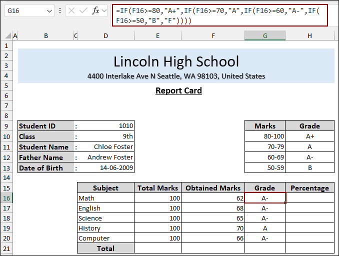
Hence, we will use a nested IF function to assign the grade based on the criteria in the grading table.
➤ In the Grade column (e.g., G16 for Math), enter the nested IF formula, hit ENTER, and pull the Fill Handle down.
=IF(F16>=80, "A+", IF(F16>=70, "A", IF(F16>=60, "A-", IF(F16>=50, "B", "F"))))
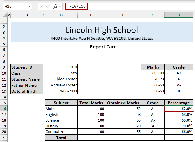
The percentage is simply the obtained marks divided by the total marks for that subject.
➤ In the Percentage column (e.g., H16 for Math), enter the formula, click ENTER, and drag down the Fill handle.
=F16/E16
Step 4: Calculating Final Results
In this final step, we will calculate the total results for all the subjects.
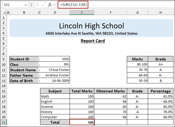
First, we will use the SUM function for the total marks and the total obtained marks.
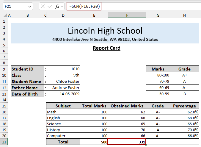
➤ In the Total row for Total Marks (e.g., E21), put the formula and click ENTER.
=SUM(E16:E20)
➤ Similarly, choose cell F21, write the formula, and press ENTER to get the Total Obtained Mark.
=SUM(F16:F20)
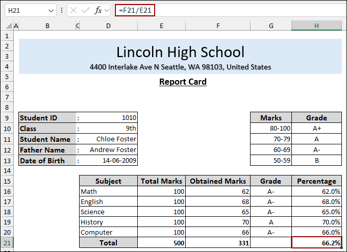
Let’s calculate the overall percentage by dividing the total obtained marks by the total marks.
➤ In the Total row for Percentage (e.g., H21), put the formula below and hit ENTER.
=F21/E21
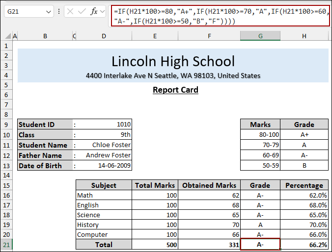
Finally, calculate the Overall Grade using the same nested IF Function. But we need to multiply the percentage by 100 to get a whole number.
➤ In the Total row for Grade (e.g., G21), enter the formula and press ENTER.
=IF(H21*100>=80, "A+", IF(H21*100>=70, "A", IF(H21*100>=60, "A-", IF(H21*100>=50, "B", "F"))))
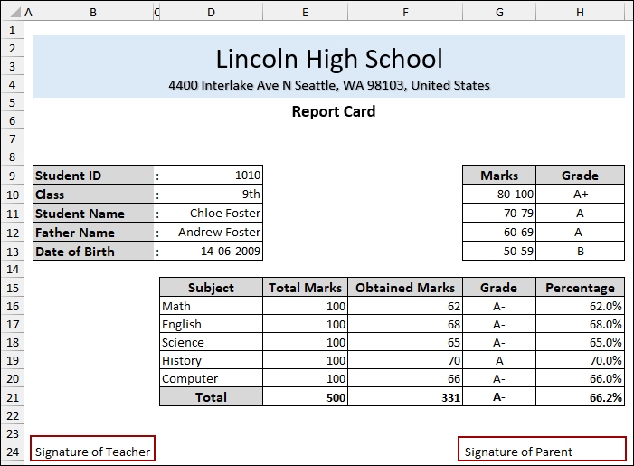
➤ Insert text labels for Signature of Teacher and Signature of Parent at the bottom of the report card.
As a result, you will have a dynamic report card in Excel that updates automatically upon selecting a new Student ID.
Frequently Asked Questions
Can I import student data from another Excel file?
Yes, you can use Power Query or the VLOOKUP function to collect student data from another workbook.
What is the best way to keep the original marks safe so teachers can’t accidentally change them?
Create a separate marks entry sheet and link it to the report card, then lock the report card sheet.
Is it possible to generate report cards for all students in PDF format automatically?
Yes, with VBA macros or Power Automate (optional), Excel can loop and export each report card individually to PDF.
Concluding Words
Above, we have covered all the steps to make a report card in Excel. The combination of the Data Validation feature with the VLOOKUP and MATCH functions is a quick way to generate a report card that dynamically links to source data. Utilizing conditional logic for grading and formatting provides a unique look to the report. If you have any questions, please don’t hesitate to share them in the comments section below.