
We often face frustrating situations where the date filter suddenly stops working, dates don’t appear in the dropdown, sorting becomes incorrect, or some entries disappear entirely. This problem usually happens due to merged cells, blank cells, text-stored dates, or inconsistent date formatting. Users commonly face these errors while filtering sales reports, project timelines, or transaction data, when Excel fails to recognize certain dates properly.
To fix the Excel date filter not working, follow these steps:
➤ Identify whether date cells are formatted correctly.
➤ Check for merged or blank date cells and unmerge or fill them properly.
➤ Reapply the filter to ensure Excel recognizes each date correctly.
In this article, we will describe troubleshooting steps for the problem where the data filter is not working in Excel through fixing text-stored dates, blank cells, unmerged cells, and restoring Excel’s filter functionality.
Enable Group Dates From the AutoFilter Menu
Sometimes the Excel date filter doesn’t show grouped months and years because the grouping feature is disabled. This method helps restore date grouping in filters so we can easily view and filter by Month or Year. We use this fix when our filter dropdown lists every individual date instead of time periods.
We have a dataset that contains a sales record for several months. But when applying the date filter on the “Order Date” column, the month and year groups do not appear. We will try to fix this problem by “Enabling the Group Date”.
Steps:
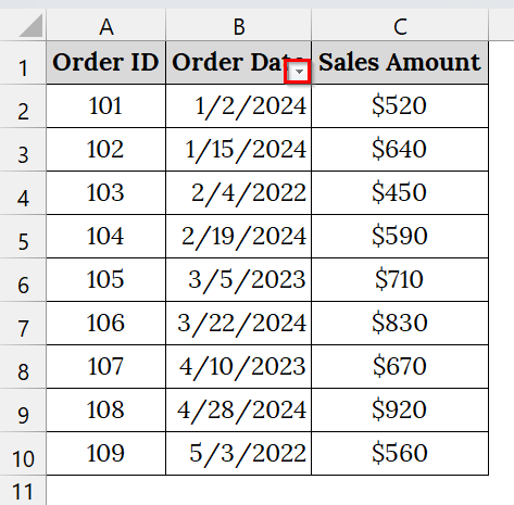
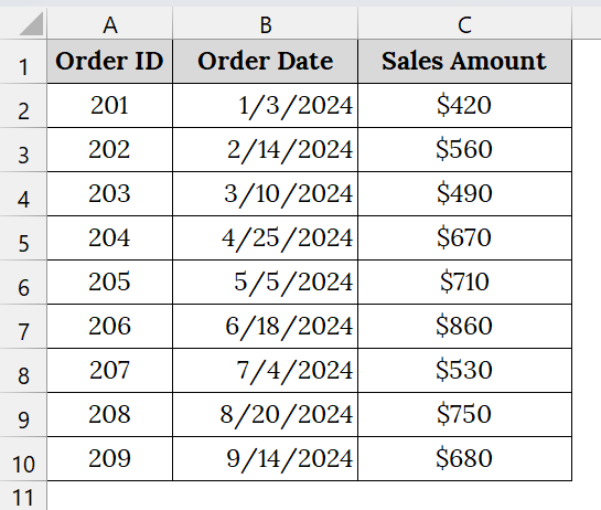
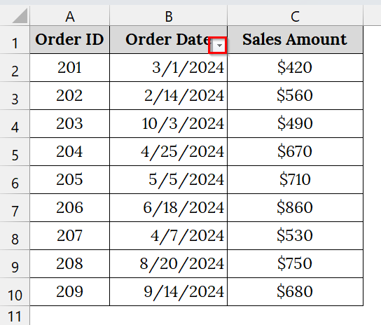
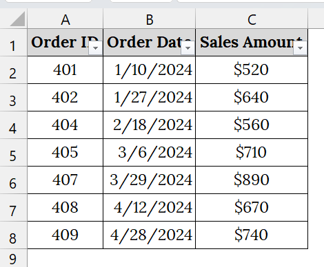
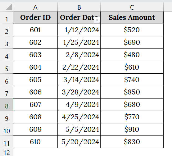
➤ Open your worksheet that contains your data, and the filter drop-down button is set. For example, we have taken a table that contains the Order ID in Column A, Order Date in Column B, and Sales Amount in Column C.
➤ Go to the File tab on the Excel ribbon. This opens the backstage view where you can access Excel’s global settings.
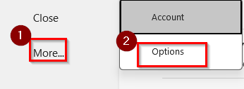
➤ Click More. Then, select Options from the bottom of the left-hand menu.
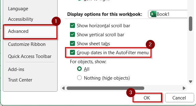
➤ From the left-side panel of the dialog box, choose Advanced.
➤ Scroll down to the section labeled Display options for this worksheet. Under that section, find and check the box that says “Group dates in the AutoFilter menu.” This setting controls whether Excel groups dates automatically when filtering.
➤ Click OK to apply the setting and close the dialog box.
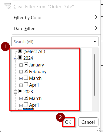
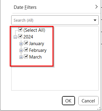
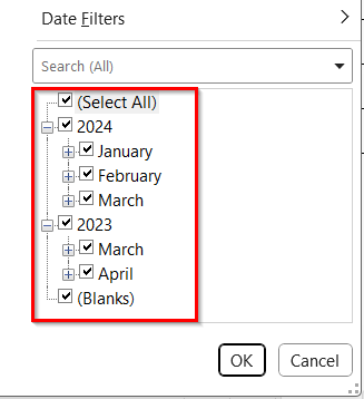
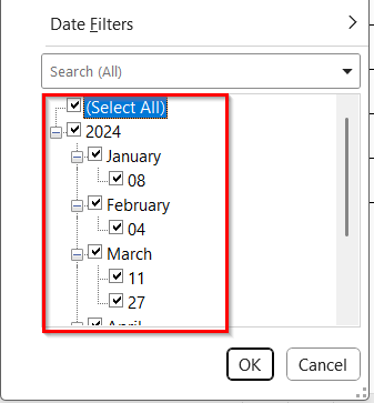
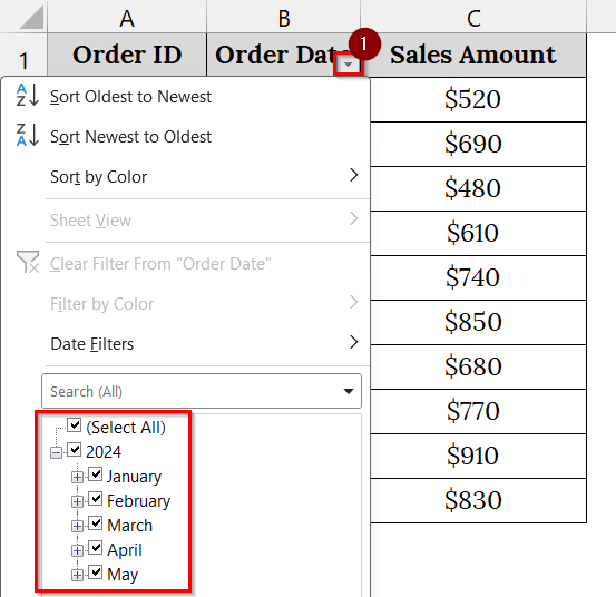
➤ Return to your worksheet, click the filter dropdown in the “Order Date” column.
➤ To verify that the dates are now grouped by Year and Month, check the preferred month and year. For example, we select January and February 2024, and March 2023.
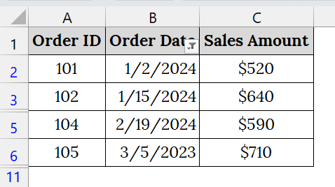
➤ Now, the result will appear.
Note:
➥ Make sure your “Order Date” column contains valid date values (not text).
➥ If it still doesn’t group, use the next method (“Convert Text to Dates”) to ensure proper date formatting.
Convert Dates Stored as Text into True Date Format
If your Excel date filter is not working, one major reason could be that the dates are stored as text instead of true date values. This happens often when data is imported from another system or typed manually with extra spaces or quotation marks. You can fix it by converting the text values to real dates so Excel can recognize and filter them properly.
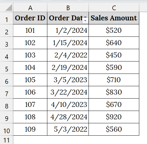
In this dataset, the Order Date column appears to contain valid dates, but Excel stores them as text because they were imported or typed incorrectly. As a result, the date filter does not work, and Excel cannot recognize the entries as true date values.
Steps:
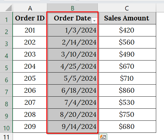
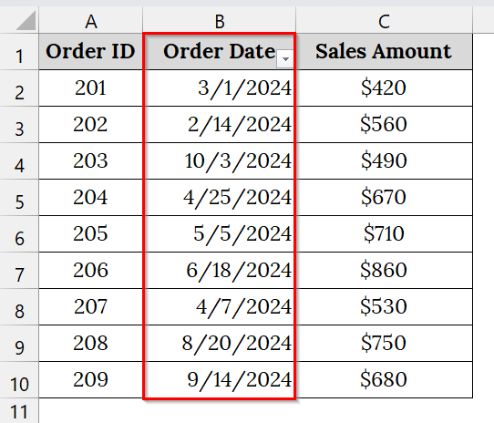
➤ Open your Excel file that contains your data. Here, we have taken a dataset that contains the Order ID in Column A, Order Date in Column B, and Sales Amount in Column C.
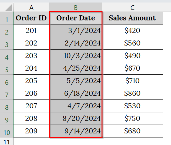
➤ Select the entire range of “Order Date” cells that contain the unrecognized date values. For example, B1:B10.
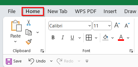
➤ Go to the Home tab on the ribbon.
➤ Locate the Number Format box in the “Number” group.
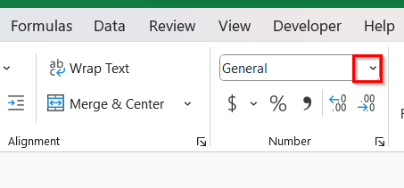
➤ Click the drop-down arrow and select Short Date or Long Date format from the list.
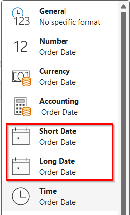
➤ At this point, the dates should be changed from text to Date format. However, if the dates remain unchanged or left-aligned, Excel is still treating them as text. To convert text to a date, we can use the Text to Columns feature.
➤ To do that, select the range A1:A10.
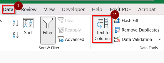
➤ Go to the Data tab → click Text to Columns.
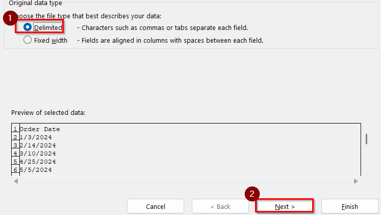
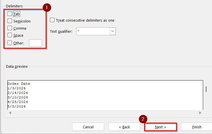
➤ In Step 1 of the wizard, select Delimited → click Next.
➤ In Step 2, uncheck all delimiters → click Next.
➤ In Step 3, select Date, and choose the correct date format (e.g., MDY). Click Finish.
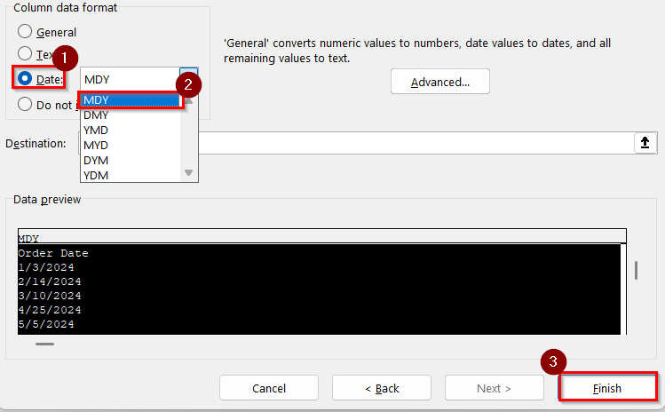
➤ After applying the conversion, Excel will recognize them as date values.
➤ Now Reapply the filter on your dataset.
➤ To do that, select the Order Date Column again.
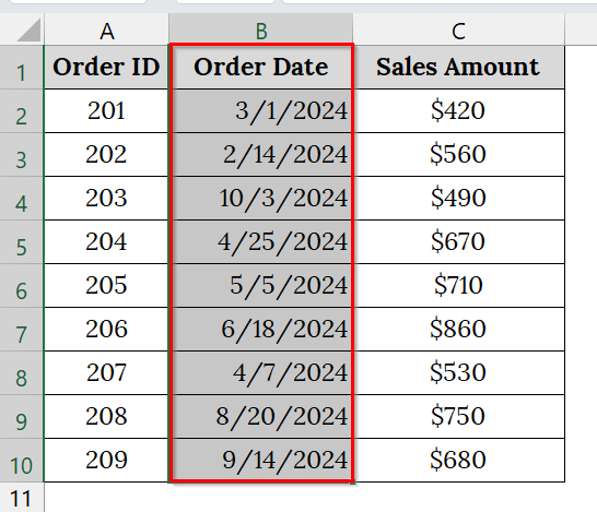
➤ Go to Data to Filter.
➤ The drop-down arrow will appear now and will work for all dates.
Use Manual Selection Technique to Ensure Filter Applies to All Rows
Sometimes the date filter doesn’t include all records; it is often because the filter range is broken by blank rows or extra spaces in the dataset. We use this fix when we notice missing records in filtered results.
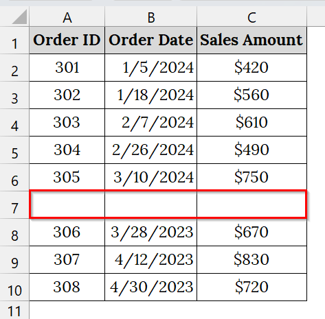
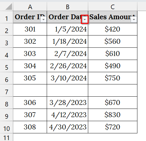
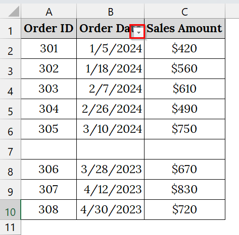
We have an Excel Workbook that contains a blank row between entries 305 and 306. Because of that, the filter may apply to the range above the blank row. The rest of the data (rows 306–309) remains unfiltered, causing missing rows when we apply sorting or filtering by date.
Steps:
➤ Check your dataset for any blank rows or gaps between records. You can do this by scrolling through your data. For example, notice a blank row at Row 7 between Order ID 305 and 306.
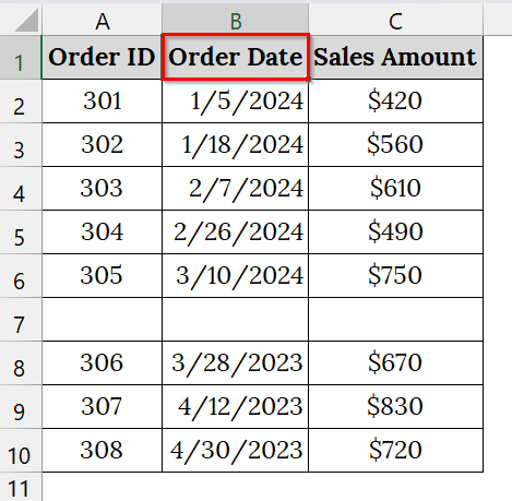
➤ Click on any cell inside your data range. For example, cell B1.
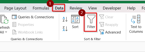
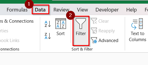
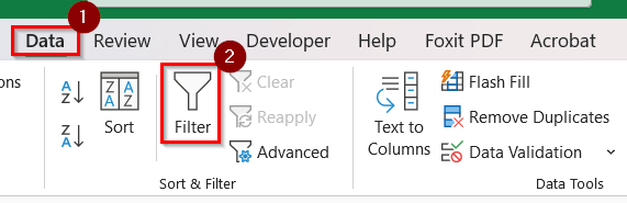
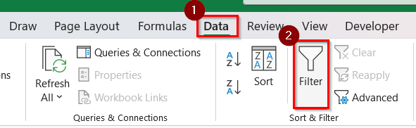
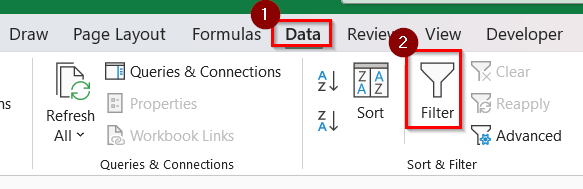
➤ Go to the Data tab → select Filter.
➤ Click on the Drop-down arrow.
➤ If your data has a break, Excel will only apply filters up to the blank row.
➤ Remove any previously applied filter by unchecking it. After that, we will apply the filter again.
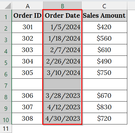
➤ Then, select all rows in the dataset manually. Manual selection ensures that the filter covers the entire selected dataset. For example, select B1:B10, including any blank rows.
➤ Now, to reapply the filter, go to Data → Filter.
➤ Click on the Drop-down arrow.
➤ Check that filter arrows appear for the full dataset, including the previously unfiltered rows.
Remove Rows with Blank Cells from the Dataset
Blank cells inside a dataset can interrupt Excel’s AutoFilter range, causing the filter to skip parts of our table. Removing these rows with bank cells restores the data’s continuity so filters can include all records. This method is good when we find gaps between rows that prevent proper date sorting or filtering.
We have a worksheet that contains blank cells scattered throughout the data table. These empty cells break the continuity of the dataset, which causes Excel’s AutoFilter or sorting feature to behave incorrectly. We will remove these blank cell-containing rows to make the filter work smoothly.
Steps:
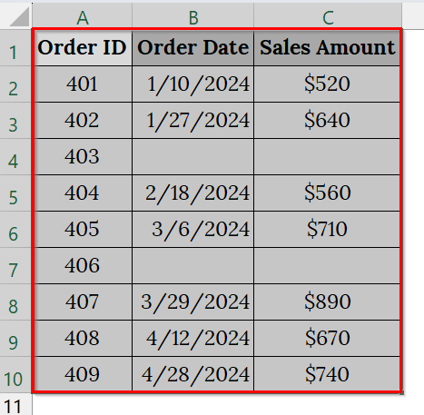
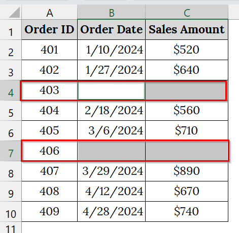
➤ Select the entire data range (A1:C10) containing both filled and blank cells.
➤ Go to the Home tab.
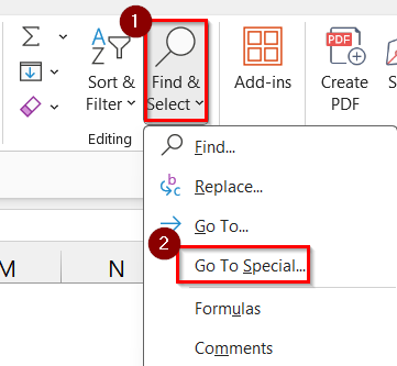
➤ Click the Find & Select dropdown in the “Editing” group → Choose Go To Special.
➤ In the Go To Special dialog box, select Blanks and click OK.
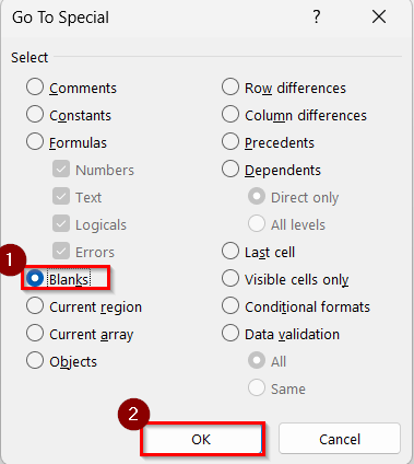
➤ This will highlight all blank cells within the selected range.
➤ Now, right-click any of the highlighted blank cells and choose Delete.
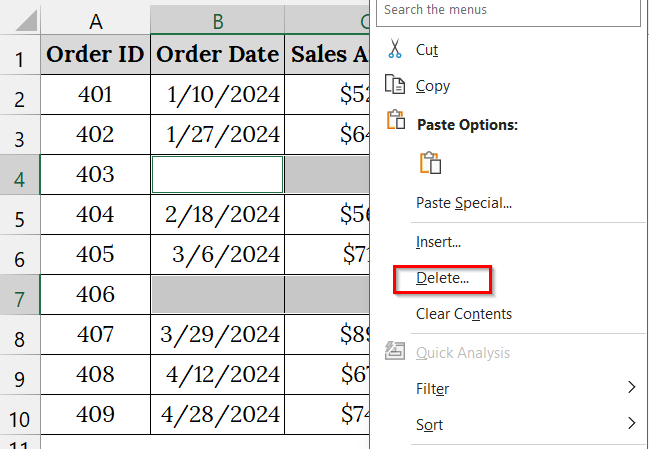
➤ In the Delete dialog, select Entire Row → click OK.
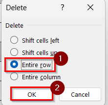
➤ This removes all blank rows at once.
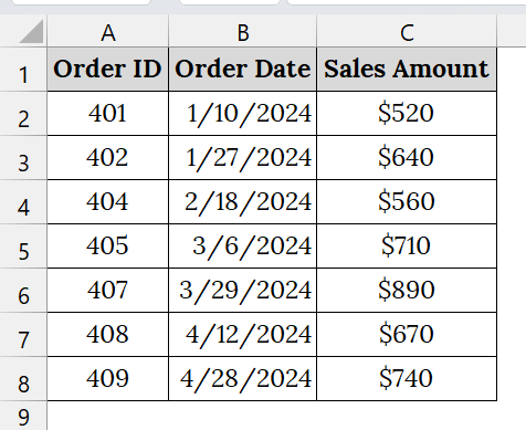
➤ Once the blank rows are deleted, your dataset becomes continuous.
➤ Reapply the filter. To do that, click any cell like A2.
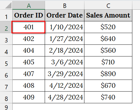
➤ Go to the Data tab → Filter.
➤ Check, the filter is working.
Unmerge Any Merged Cells in the Date Column
Merged cells often disrupt Excel’s filtering and sorting features because they prevent each row from being recognized as a separate entry. This method helps us unmerge date cells, fill missing values, and restore the filter’s full functionality. This method is good for datasets where merged cells were used for grouping, but now need to be analyzed row by row.
We have an Excel workbook containing several date cells that are in a merged condition. Excel’s AutoFilter cannot properly recognize or sort merged cells, which leads to incomplete filtering or sorting errors.
Steps:
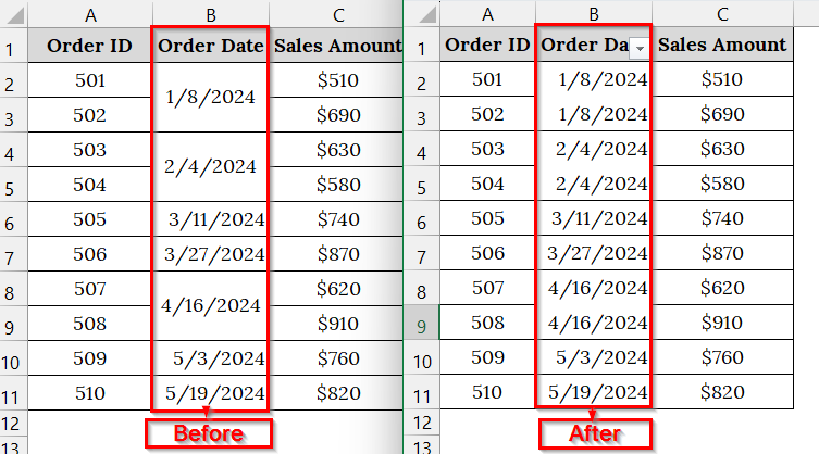
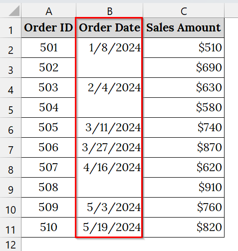
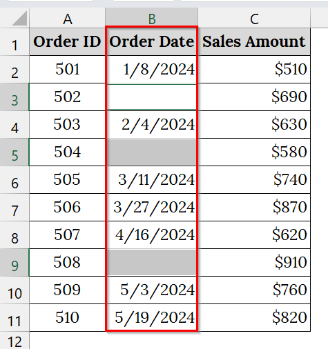
➤ Open your Excel sheet that contains the merged cell. For example, we have taken a table that contains merged cells in Column B, named Order Date.
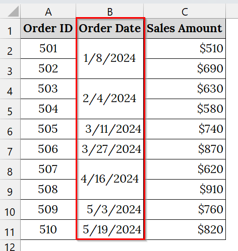
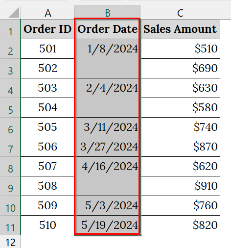
➤ Select the entire dataset containing merged cells (A1:C11).

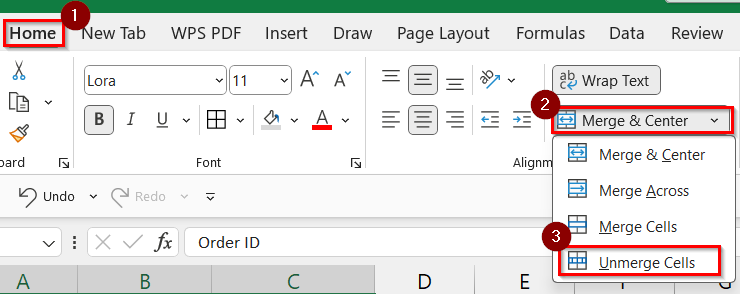
➤ Go to the Home tab → In the Alignment group, click the Merge & Center dropdown → Choose Unmerge Cells.
➤ After unmerging, notice that only the first cell in each merged block retains the date. The others become blank.
➤ To fill the blank cells. Select the “Order Date” column again.
➤ Press the keyboard shortcut Ctrl + G and then click Special.
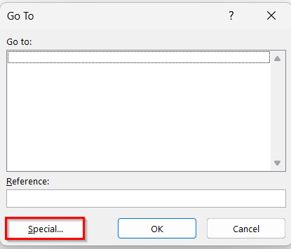
➤ Choose Blanks → Click OK.
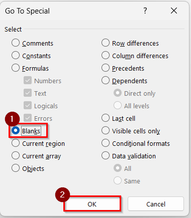
➤ This will select only the blank cells under unmerged dates.
➤ Without deselecting, in the formula bar, type the previous cell reference manually.
➤ Here we have typed =B2, because B2 is the cell above the first blank.
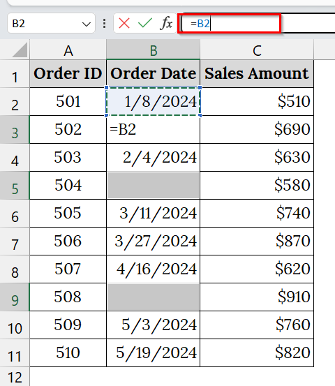
➤ Now press Ctrl + Enter to fill all blanks with the date above.
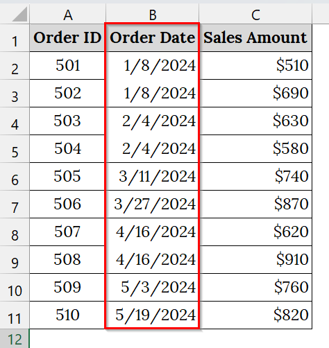
➤ Now, reapply the filter. To do that, select the “Order Date” column.
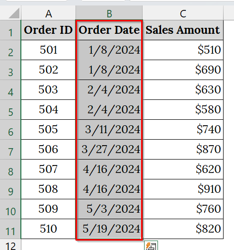
➤ Go to Data → select Filter.
➤ You will now be able to sort and filter all records without missing entries.
Note:
➥ Avoid using merged cells in data tables intended for analysis.
➥ Always fill down dates after unmerging to maintain dataset consistency.
➥ You can also use Excel’s Find & Select → Replace Blanks feature as an alternative to the “fill-down” formula method.
Unprotect the Worksheet (If It’s Protected)
If your Excel date filter is unresponsive or greyed out, the worksheet may be protected. Worksheet protection restricts editing and disables filtering or sorting actions.
We have a worksheet that has been protected to prevent users from editing or accidentally deleting formulas. However, when protection is active, Excel disables features like sorting and filtering. As a result, clicking the filter arrows in the “Order Date” column does nothing, and the date filter appears to be “not working.”
Steps:
➤ Open your worksheet. Try clicking the filter dropdown on the “Order Date” column.
If it is greyed out, that means your worksheet is protected.
➤ Go to the Home tab.
➤ In the Cells group, click the Format dropdown.
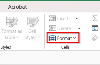
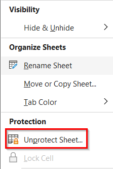
➤ From the dropdown menu, click Unprotect Sheet. If the sheet is password-protected, a dialog box will appear asking you to enter the password.
➤ Click on the drop-down arrow to check if the filter feature is working.
Frequently Asked Questions
Why is my Excel date filter missing certain dates?
It usually happens when some date cells are merged or stored as text instead of using the proper date format.
How do I convert text-stored dates into real dates in Excel?
Use the Text to Columns tool or the DATEVALUE function to convert text-based dates into valid date values.
Can merged cells affect the date filter?
Yes. Excel treats merged cells as a single record, so unmerging them ensures that each row has its own filterable date.
What should I check first when my date filter doesn’t work?
Begin by verifying your date column format and unmerging any merged cells.
Concluding Words
When your Excel Date Filter is not working, the problem almost always lies in improper formatting or merged cells. We have described six effective methods that should fix your problem in no time. We have uploaded the Excel files and dataset used in this article so that you can download and practice those troubleshooting steps beforehand.