A search box in Excel helps you quickly find and display data without scrolling through multiple sheets manually. Instead of manually searching in tabs or using Ctrl + F repeatedly, you can build a simple search tool to look up information across several sheets instantly.
This is especially useful when you manage large datasets split into multiple sheets, such as quarterly sales, regional reports, or department data. A well-designed search box improves navigation, reduces time spent searching, and makes your workbook much more user-friendly.
In this guide, you’ll learn how to create a search box in Excel for multiple sheets using a dynamic method.
Here’s how to build a search box in Excel that searches through multiple sheets:
➤ Open your dataset in Excel and convert it into a Table on each sheet such as Sales1, Sales2, and Sales3.
➤ Next, create a new sheet and name it Search. This is where we’ll design the search box interface.
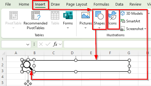
➤ Go to Insert >> Shapes and draw a rectangular shape that will act as your search box.
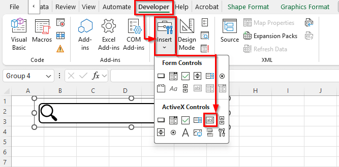
➤ Go to the Developer tab and click Insert >> Text Box (ActiveX Control).
➤ Draw the Text Box inside the shape you created earlier.
➤ Prepare a result table to display matches.
➤ Select the first cell under your result headers. For example, B7 in the Search sheet.
➤ Enter the following formula:
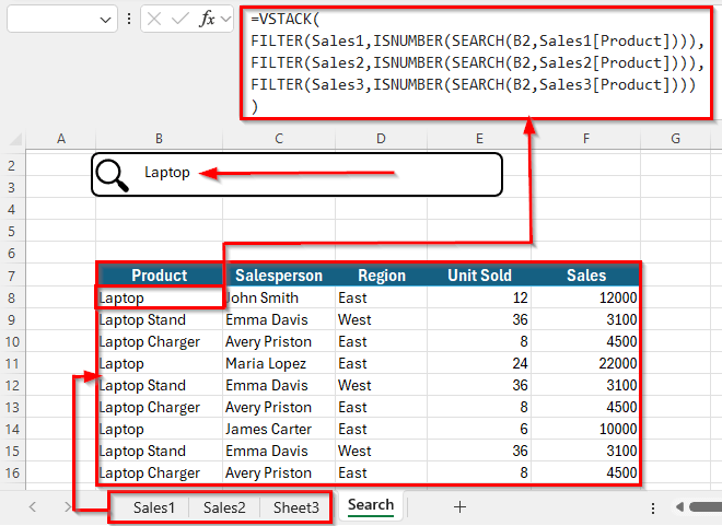
=VSTACK(FILTER(Sales1,ISNUMBER(SEARCH(B2,Sales1[Product]))),FILTER(Sales2,ISNUMBER(SEARCH(B2,Sales2[Product]))),FILTER(Sales3,ISNUMBER(SEARCH(B2,Sales3[Product]))))
➤ Press Enter. You’ll now see the Search sheet will display a combined list of all rows from Sales1, Sales2, and Sales3.
➤ Now, whenever you type a product name or part of it in the search box, the result table instantly updates with all matching rows across all three sheets.
Steps to Create a Dynamic Search Box for Multiple Excel Sheets
Let’s prepare a sample workbook with three sheets named Sales1, Sales2, and Sales3. Each sheet contains product sales data where Column A stores the Product Name, Column B shows the Salesperson, Column C lists the Region, Column D shows the Units Sold, and Column E displays the Sales amount.
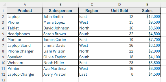
Use the same structure for Sales2 and Sales3 but with different data values. We’ll use this dataset to demonstrate the dynamic search methods in the next sections
In this method, we’ll build a fully dynamic search box that instantly filters and displays matching results as you type. It’s one of the easiest and most powerful ways to create a responsive search feature in Excel.
We’ll use the FILTER function with a search condition and set up a simple interface to let users search any product name dynamically.
Step 1: Set Up the Search Input Area
First, choose a location in your worksheet where users will type the search keyword.
Here’s how to do it:
➤ Open your dataset in Excel and convert it into a Table on each sheet such as Sales1, Sales2, and Sales3.
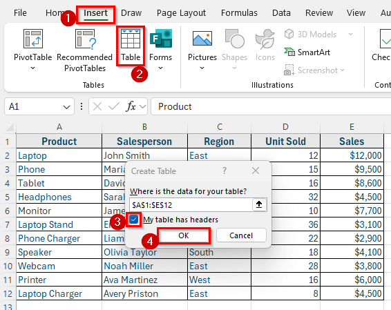
➤ Select your dataset range and click Insert >> Table >> My table has headers >> Ok.
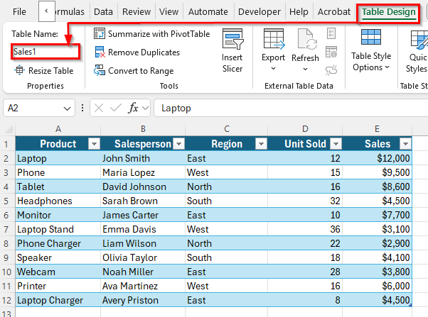
➤ Go to Table Design and give your table a suitable name. For example: Sales1 on the first sheet, Sales2 on the second, and Sales3 on the third.
➤ Next, create a new sheet and name it Search. This is where we’ll design the search box interface.
➤ Go to Insert >> Shapes and draw a rectangular shape that will act as your search box.
➤ To give it a professional look, go to Icons and select a search icon from the dropdown and place it on the left side of the shape.
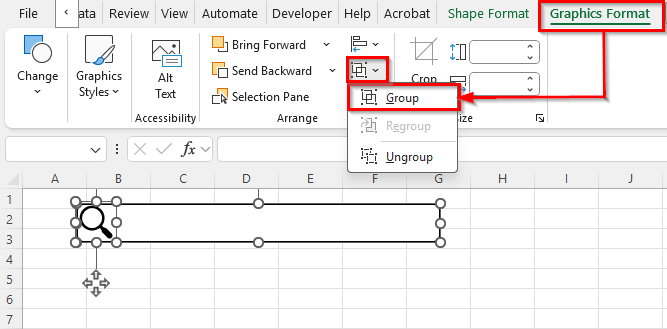
➤ Finally, select both the shape and the icon, then go to Graphics Format >> Group to combine them. This grouped shape will serve as the search input box for users.
Step 2: Add an ActiveX Search Box for User Input
To make the search box functional and user-friendly, you can insert an ActiveX Text Box instead of relying only on a shape. This will allow users to type search keywords directly into the search box.
Here’s how to do it:
➤ Go to the Developer tab and click Insert >> Text Box (ActiveX Control).
➤ Draw the Text Box inside the shape you created earlier.
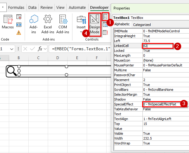
➤ Right-click it and select Properties.
➤ Set the LinkedCell property to B2 (this is where the typed search text will appear) and SpecialEffect to 0 – fmSpeacialEffectFlat to give it a clean, modern look.
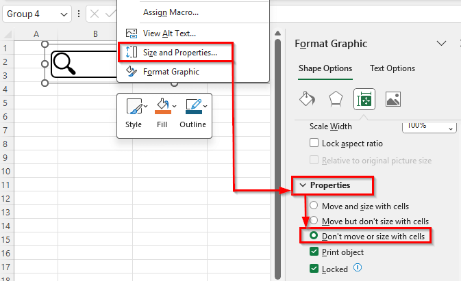
➤ Again right-click on the Text box and select Size and Properties from the context menu.
➤ Under the Properties dropdown, set the option to Don’t move or size with cells so the search box stays fixed even if you resize or modify the worksheet.
Step 3: Prepare a Result Table to Display Matches
Now that the search input box is ready, the next step is to create a dedicated area where the search results will appear. This table will automatically update based on the keyword entered in the search box.
Here’s how to do it:
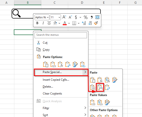
➤ Open your sheet Sales1 and copy the header section only.
➤ Now, go to the Search sheet and select a blank cell, right-click on it and select Paste Special >> Keep Source Column Widths.
Step 4: Use the FILTER with VSTACK Function to Return Results for Multiple Sheets
With the result table ready, it’s time to make it dynamic. We’ll use the FILTER function to pull matching records from all three sheets based on the keyword entered in the search box. Then we’ll stack the results into a single table using the VSTACK function.
Here’s how to do it:
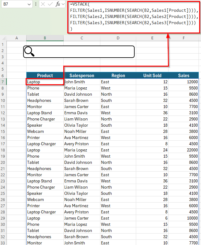
➤ Select the first cell under your result headers. For example, B7 in the Search sheet.
➤ Enter the following formula:
=VSTACK(FILTER(Sales1,ISNUMBER(SEARCH(B2,Sales1[Product]))),FILTER(Sales2,ISNUMBER(SEARCH(B2,Sales2[Product]))),FILTER(Sales3,ISNUMBER(SEARCH(B2,Sales3[Product]))))
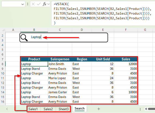
➤ Press Enter. You’ll now see the Search sheet will display a combined list of all rows from Sales1, Sales2, and Sales3.
➤ Now, whenever you type a product name or part of it in the search box, the result table instantly updates with all matching rows across all three sheets.
Step 5: Expand to Multi-Column Search with a Combined Formula
You can make the search more powerful by checking multiple columns at once. For example, searching both Product and Salesperson columns.
Here’s how to do it:
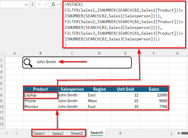
➤ Select cell B7 in the Search sheet.
➤ Enter the following formula:
=VSTACK(FILTER(Sales1,ISNUMBER(SEARCH(B2,Sales1[Product]))+ISNUMBER(SEARCH(B2,Sales1[Salesperson]))),FILTER(Sales2,ISNUMBER(SEARCH(B2,Sales2[Product]))+ISNUMBER(SEARCH(B2,Sales2[Salesperson]))),FILTER(Sales3,ISNUMBER(SEARCH(B2,Sales3[Product]))+ISNUMBER(SEARCH(B2,Sales3[Salesperson]))))
➤ Press Enter.
➤ Now, the Search sheet will display a combined list of all rows from Sales1, Sales2, and Sales3 where the search term appears in either the Product or Salesperson column. The results will update automatically whenever you type a new keyword in the search box.
Frequently Asked Question
How do I create a search box that searches across multiple sheets in Excel?
To create a search box that scans data across multiple sheets, use the FILTER and VSTACK functions together. First, build a search input field using an ActiveX Text Box or a cell reference. Then, write a formula like:
=VSTACK(FILTER(Sales1,ISNUMBER(SEARCH(B2,Sales1[Product]))),FILTER(Sales2,ISNUMBER(SEARCH(B2,Sales2[Product]))),FILTER(Sales3,ISNUMBER(SEARCH(B2,Sales3[Product]))))
This formula combines results from all sheets and displays matching records in one place.
Can I search multiple items in multiple sheets with one search box?
Yes. You can expand your FILTER formula to include multiple columns using the + operator with ISNUMBER and SEARCH functions. For example, use this following formula:
=VSTACK(FILTER(Sales1,ISNUMBER(SEARCH(B2,Sales1[Product]))+ISNUMBER(SEARCH(B2,Sales1[Region]))),FILTER(Sales2,ISNUMBER(SEARCH(B2,Sales2[Product]))+ISNUMBER(SEARCH(B2,Sales2[Region]))),FILTER(Sales3,ISNUMBER(SEARCH(B2,Sales3[Product]))+ISNUMBER(SEARCH(B2,Sales3[Region]))))
This will return rows if the search term appears in either the Product or Region column in any sheet.
How do I make the search box show results instantly as I type?
If you use an ActiveX Text Box linked to a cell, Excel recalculates formulas each time the cell changes. That means the FILTER results will update automatically as you type. This makes the search experience dynamic and real-time.
Wrapping Up
Building a dynamic search box across multiple sheets makes it much easier to explore large Excel workbooks. Instead of jumping between tabs or using multiple filters, you can type a keyword once and see all matching results combined into one place.
Using functions like FILTER, SEARCH, ISNUMBER and VSTACK keeps the solution fully formula-based, while adding an ActiveX text box improves the user experience.
With this setup, you can quickly search products, salesperson, regions, or any other field across several sheets and keep your workflow organized and efficient.