In data analysis, we often need to find values of significant data points in a dataset. For example, in a business, you might have some product names and want to look up the stock level of that product. To do that, Microsoft Excel allows you to look up a value in a column and return the value of another column. In this article, we will learn the process using various formulas and functions.
➤ Select the cell where you want to get the value.
➤ Write this formula:
=VLOOKUP(“John Smith”,A2:E12,3,FALSE)
➤ Replace “John Smith” with the value you are looking up, A2:E12 with the cell range, and 3 with the other column from where you want the value to return from.
➤ Press Enter.
In this article, we will learn the explanation of this method and go through some more formulas so that you can choose the suitable one for your job. Therefore, keep reading to learn and apply them to your use case.
Quick Video Tutorial: Lookup in One Columns & Return Value from Another Column
Using the VLOOKUP Function
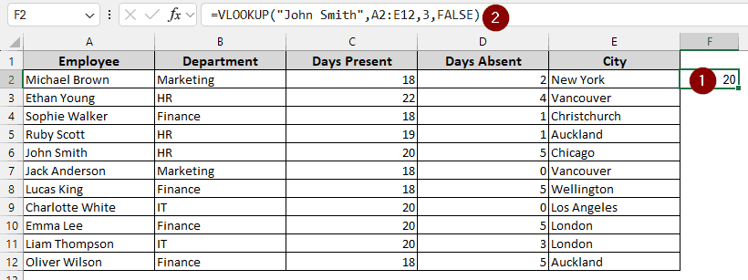
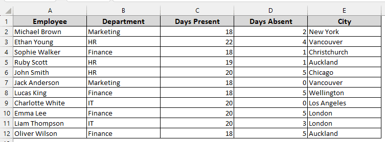
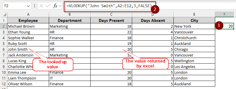
In our example dataset, we have some records of employees including the departments they work in, how many days they were present or not, and what city they are from. An HR manager might want to know how many days a particular employee worked to issue their salary.
However, when there are hundreds of employees in a company, it is not easy to find the record of a single employee. This article will teach you how to do that easily.
The VLOOKUP function is a well-known function in Microsoft Excel. It has been around a long time, and it gets the job done. Here is how to use it to look up a value in one column and return a value from another.
Steps:
➤ Go to the cell where you want to see the value.
➤ Write this formula:
=VLOOKUP(“John Smith”,A2:E12,3,FALSE)
➤ Press Enter after setting the parameters properly and excel will return the value.
Using the XLOOKUP Function
Although the VLOOKUP function has been there for a while, Microsoft has introduced a new version of the function called XLOOKUP that is less confusing and works better. However, you will need at least Excel 2021 to use this function. Older versions of Office will not work, although you can open a file created using this function on Excel 2016/2019/365.
Steps:
➤ Just like before, select the output cell for the value.
➤ Enter this formula:
=XLOOKUP(“John Smith”, A2:A12, C2:C12)

Using INDEX-MATCH Formula
If those two functions didn’t meet your needs, and you want something out of the regular functions, this solution is for you. We are going to make the use of INDEX and MATCH functions together to do the job.
Steps:
➤ Go to the output cell, and enter this formula:
=INDEX(A1:E12,MATCH(“John Smith”,A1:A12,0),3)

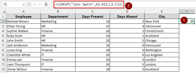
Using the LOOKUP Function
Finally, if you have a really old Microsoft Office version, you have no other choice but to use the LOOKUP function. It is very easy to use, but Microsoft does not recommend this function to be used in newer spreadsheets.
Steps:
➤ This function works almost exactly like the newest XLOOKUP function. Use this formula:
=LOOKUP(“John Smith”,A2:A12,C2:C12)
Frequently Asked Questions
How to use VLOOKUP in Excel to return a value from another sheet?
Modify the formula like this
=VLOOKUP(“John Smith”, Sheet2$A2:E12,3,FALSE)
Here, Sheet2 is the other sheet where the data belongs.
Can VLOOKUP match 2 values?
No. However, you can create a separate column to create unique values, and then match values from that column.
Does VLOOKUP return yes or no?
No. However, you can combine the function with IF and ISNA functions to return yes or no. The formula should be written like this:
=IF(ISNA(VLOOKUP(“John Smith”, A2:E12,3,FALSE)), “No”, “Yes”)
What are the three types of lookup in Excel?
The three types of lookup are XLOOKUP, VLOOKUP, and HLOOKUP. XLOOKUP works for any type of lookup, while VLOOKUP and HLOOKUP work with vertical and horizontal lookup, respectively.
How to apply HLOOKUP in Excel?
Use the formula like this:
=HLOOKUP(“Employee”, A1:E12, 6, FALSE)
The lookup value must be in the first row.
Wrapping Up
By reading this article, you have learned four ways to look up a value in a column and return the value of another column in Excel. Use the practice file for exercising and mastering the formulas. Don’t forget to leave a comment if you found this article useful.