
Dynamic arrays in Excel allow formulas to automatically return multiple values or single values based on a range of cells without needing to copy formulas manually. Dynamic array is widely used for tasks like filtering lists, sorting data, or generating unique values dynamically. It saves time, reduces errors, and makes spreadsheets more flexible and responsive to changes in source data.
To use dynamic array in Excel you can follow these example steps:
➤ Select the cell where we want the results to appear using a dynamic array.
➤ Enter a dynamic array formula. Such as formulas with SORT, FILTER, or UNIQUE function.
➤ Press Enter. Excel will automatically show the results into adjacent cells for the whole array.
In this article, we will explain what a dynamic array is, how it works in Excel, examples of common formulas, and practical tips for using them effectively.
What Is a Dynamic Array in Excel?
Dynamic Arrays are resizable arrays that calculate automatically and return values into multiple cells based on a formula entered in a single cell. Excel automatically adjusts the output range as the source data changes. It is good for tasks like extracting unique lists, sorting data instantly, or applying conditions with the FILTER function.
Using the UNIQUE Function with Dynamic Array to Extract Values
The UNIQUE function in Excel is a dynamic array based function that returns a list of distinct values from a range or array. We can use it when we need to remove duplicates and keep our dataset automatically updated.
We have a dataset that tracks the monthly sales data for our team. We want a quick, automatic updating list of all unique products sold without manually filtering or removing duplicates. We will use Dynamic array functions like UNIQUE to quickly create a list and adjust automatically if new products are added or edited.
Steps:
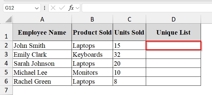
➤ Open your excel file. We have the following columns: Product, Salesperson, and Units Sold.

➤ Select the cell where the Unique list will appear (such as D2).
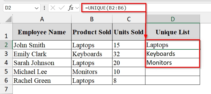
➤ Type the following formula and press Enter–
=UNIQUE(B2:B6)
Excel will display the unique product names in cells D2:D6
Combining Several Dynamic Array Functions in One Formula
Combining several dynamic array functions means combining multiple array functions (such as FILTER, SORT, and UNIQUE in a single Excel formula. We use it when we want to process and format our dataset without extra helper columns.
We have a table that represents fruit sales from different regions in a grocery distribution business. We want to filter only the East region’s sales, sort them from highest to lowest, and list each product only once. We will use multiple dynamic array functions in Excel.
Steps:
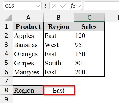
➤ Prepare the dataset. We have the following columns: Product, Region, Sales. We have named cell A8 as Region.
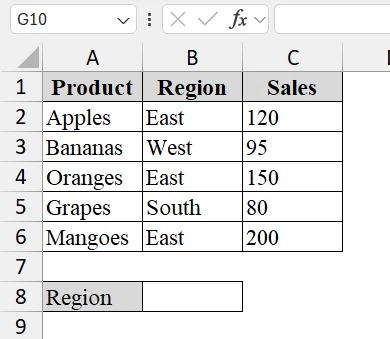
➤ Identify the target region for which we want the results. For example, if we want products sold in the East region, we will enter “East” in cell B8 for easy reference.
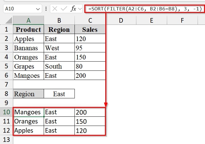
➤ Enter the combined formula in cell A10:
=SORT(FILTER(A2:C6, B2:B6=B8), 3, -1)
➥ SORT(..., 3, -1) → Sorts the filtered results by the 3rd column (Sales) in descending order.
We will have the filtered result now.
Using VLOOKUP Formula with Dynamic Arrays
We can use the dynamic VLOOKUP function combined with the FILTER function to list all matching values for a given search term. It is useful when we want to retrieve multiple related records (e.g., all projects for an employee) from a dataset.
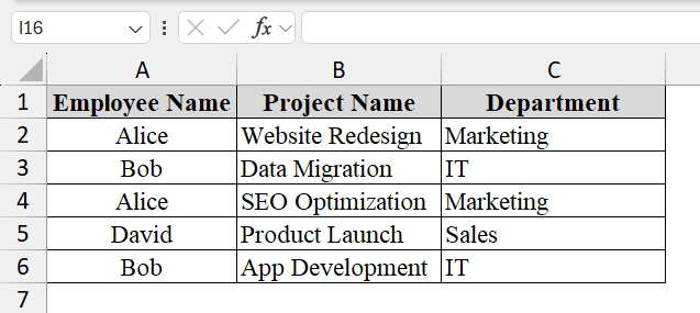
We have a table that tracks multiple projects for each employee. We want to type in an employee’s name once (e.g., “Alice”) and instantly see a list of all projects they are working on without manually filtering. We will use Excel’s dynamic array functions with a modified VLOOKUP approach.
Steps:
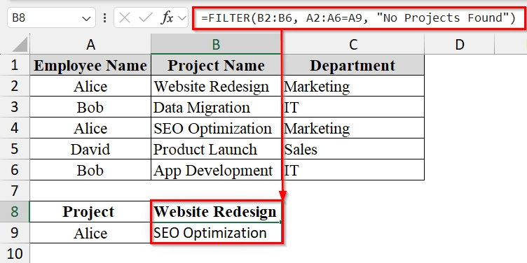
➤ Open your dataset where you want to perform the dynamic array formula. Here we have taken the following columns: Employee Name, Project Name, Department and Project.
➤ Set up the search criteria cell. For example, in cell A9, type the employee name we want to search for (“Alice”).
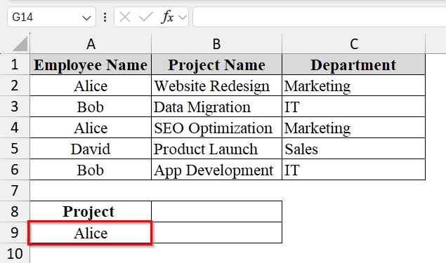
➤ In cell B8, enter the following formula. Click Enter, Excel will automatically “spill” the matching values into the rows below B8.
=FILTER(B2:B6, A2:A6=A9, "No Projects Found")
➥ A2:A6=D2 → Logical test to match the Employee Name with the search value in D2.
➥ "No Projects Found" → Message shown if there’s no match.
Using XMATCH Function in Excel with Dynamic Arrays
The XMATCH function in Excel is used to return the position of a value in a range or array. It is an improvement over the traditional MATCH function and works smoothly with dynamic arrays. We can use XMATCH when we need to quickly locate an item’s position in a dataset, such as finding where a specific product appears in a product list.
We have a dataset that represents a company’s product sales across different regions. We want to find the position of any product in the list. By using XMATCH, we can find it.
Steps:
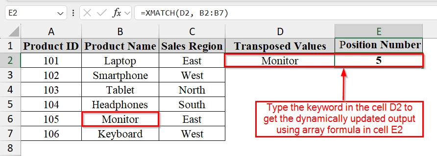
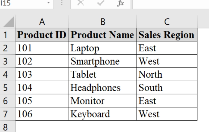
➤ Enter the dataset in Excel. For example, in Column A (Product ID), Column B (Product Name), and Column C (Sales Region).
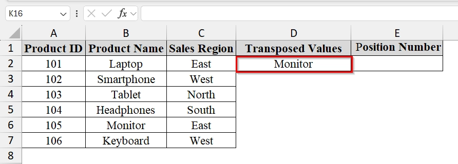
➤ Choose the value we want to find the position of. For example, in cell D2, type the product name “Monitor“.
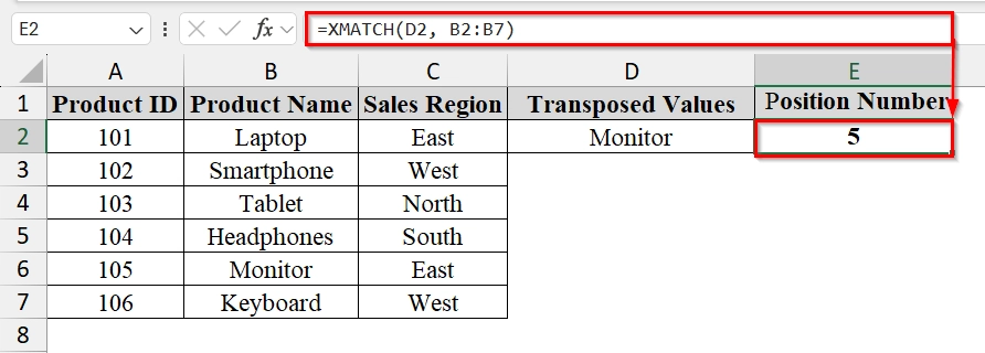
➤ In cell E2, enter the formula:
=XMATCH(D2, B2:B7)
➥ B2:B7 = the range of product names
This formula will return the position number of the product in the list.
Frequently Asked Questions
Do dynamic arrays work in all versions of Excel?
No. Dynamic arrays are available in Excel 365, Excel 2021, and Excel for the web.
What happens if the spill range is blocked?
You will get a #SPILL! error, meaning something is obstructing where the array wants to output its results.
Can I use dynamic arrays with traditional functions?
Yes, many older functions can be combined with dynamic array formulas for more flexible results.
Concluding Words
We can make dynamic arrays in various ways. The benefit of using dynamic array is the output is dynamically updated as we change the input. Download the excel file that contains all the dataset we have used in this article and practice these methods. Let us know which method worked best for you in the comment section below.