
Excel array formulas are a powerful way to perform multiple calculations at once, returning either a single value or multiple values. They are used for tasks like summing based on multiple conditions, finding unique values, or performing matrix operations. These formulas are good for anyone dealing with complex datasets.
To use Excel array formula examples, follow these steps:
➤ Select the cell(s) where we want the result to appear.
➤ Enter the array formula.
➤ Press Ctrl + Shift + Enter (for older versions) or simply Enter (for Excel 365/2021).
In this article, we will cover the meaning of array formulas, practical examples for everyday Excel tasks, such as calculating the total marks, determining the highest marks, calculating the average etc.
What Is an Excel Array Formula?
Excel array formula is a type of formula that performs multiple calculations on one or more items in an array (a range of cells) and returns a single or multiple results. They can work horizontally, vertically, or both. Modern Excel automatically handles array results without special keystrokes, while older versions require pressing Ctrl + Shift + Enter to identify the formula as an array formula.
Calculating the Total Marks of Students Using an Array Formula
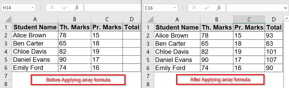
The array formula can calculate total marks for multiple students at once by adding two or more columns. This method is good when we have large datasets, such as marks for many students, and want to avoid typing formulas row-by-row.
We have a table that contains the Theory Marks and Practical Marks of students in two separate columns. We want to get the Total Marks for each student. We will calculate the total marks by using an Excel array formula.
Steps:
➤ Select the range where we want the results to appear. In this case, select cells D2:D6 where the total marks will be displayed.
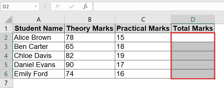
➤ In the formula bar, enter:
=B2:B6 + C2:C6
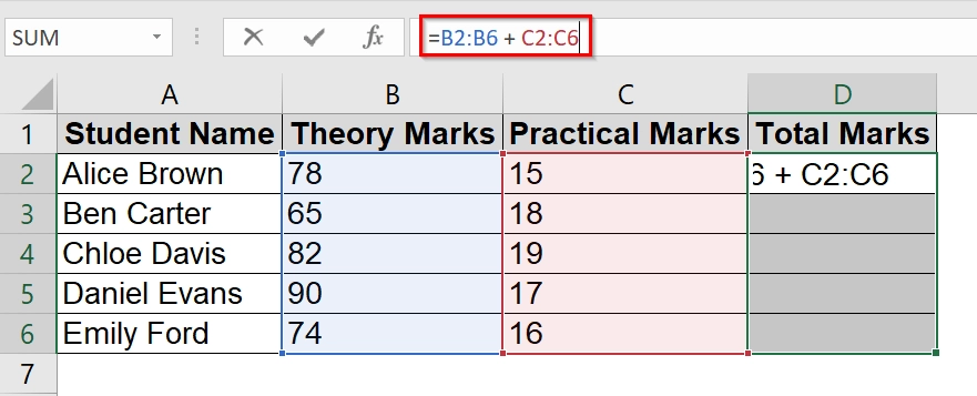
➤ Enter the formula as an array formula.
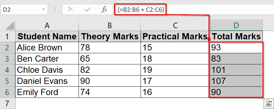
➥ In Excel 365 or Excel 2021: Simply press Enter and the results will spill automatically into D2:D6.
➥ In older Excel versions: Press Ctrl + Shift + Enter instead of just Enter . Curly braces {} will appear around the formula, indicating it as an array formula.
Determining the Highest Marks Obtained Using Array Formula
Another Array formula is Excel’s MAX function. It is used to find the largest value in a given range of cells. We can use it when we have multiple columns of numeric data such as scores, prices, or measurements and we want to know the highest value overall.
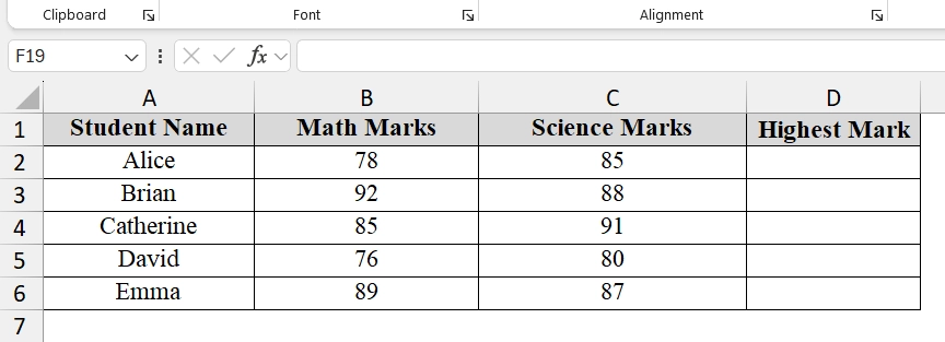
We have a worksheet that contains Math and Science marks for 10 students of a school. We want to determine the single highest mark obtained across both subjects combined. By using an array formula with MAX function, we will find this without manually scanning the list.
Steps:
➤ Open the Excel sheet containing the data. For example, the Math marks are in Column B and Science marks are in Column C and Highest Mark in Column D.
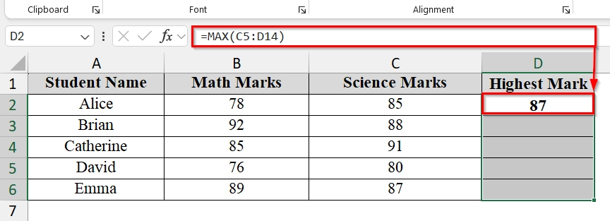
➤ Select the cell where we want to display the highest mark between C5 to C7. For example, select cell D2 to store the result. Type the formula:
=MAX(C5:D14)
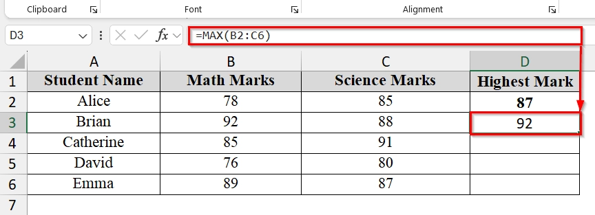
➤ Select cell D3 to store the highest result among (B2: C6) . Type the following formula in cell D3 and Press Enter.
=MAX(B2:C6)
Applying Array Formula with Multiple Criteria
An array formula with multiple criteria allows us to perform calculations on a dataset where more than one condition must be met. This method is widely used when we need results filtered by two or more rules, such as summing sales for a specific person in a specific region.
We have a dataset that represents a small company’s regional sales tracking. We want to quickly find the total sales for a specific salesperson in a specific region without manually filtering data. Using an array formula, we will sum values meeting two conditions: the salesperson’s name and the region.
Steps:
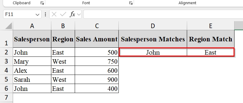
➤ Open your dataset. We have Column A: Salesperson; Column B: Region; Column C: Sales Amount, Column D Salesperson Matches and Column E Region Match.
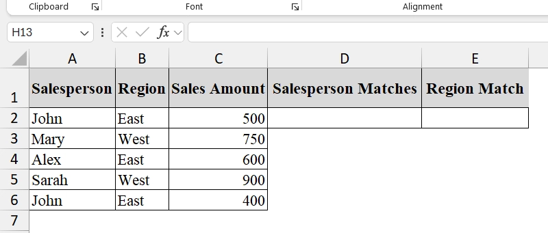
➤ Decide the criteria. For example, we want Salesperson = “John” and Region = “East”. Place these criteria in separate cells for easy reference:
- Cell D2: “John”
- Cell E2: “East”
➤ Select the output cell where we want the result (e.g., C7 ).
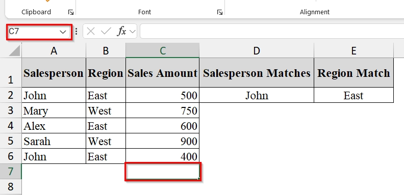
➤ Enter the array formula in cell C7. Press Enter, cell C7 will show the highest amount .
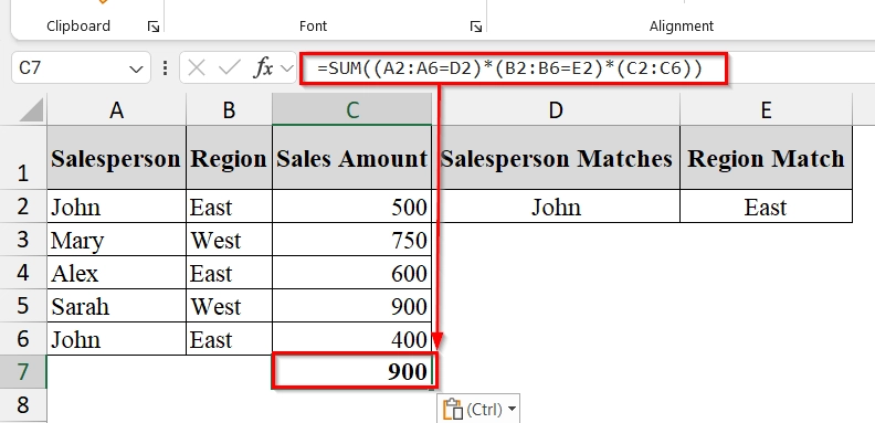
=SUM((A2:A6=D2)*(B2:B6=E2)*(C2:C6))
➥ (B2:B6=E2) checks if the region matches “East”.
➥ (C2:C6) contains the sales values.
➥ Multiplying these together keeps only the sales that match both conditions, and SUM adds them up.
Calculating the Average of the Positive Numbers Using an Array Formula
We can use array formulas to calculate the average of only positive numbers in a given dataset. It is useful when your data contains both positive and negative values, but you want to ignore the negatives.
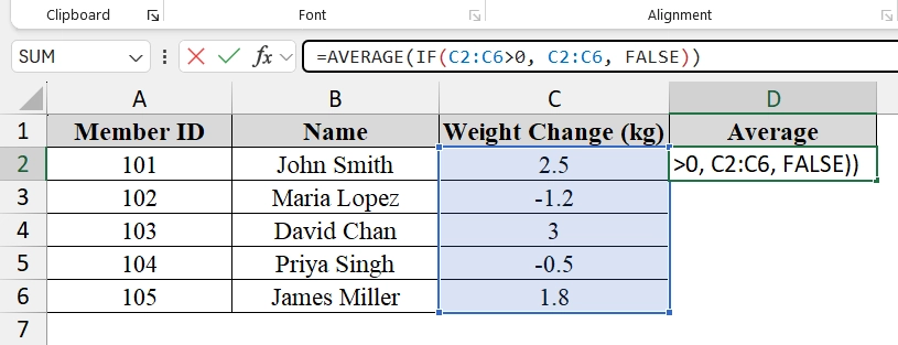
We have a table that represents a realistic gym tracking scenario where not all members have gained weight. We will calculate the average gain ignoring all negative changes using an Array formula.
Steps:
➤ Enter the data in an Excel table with at least one numeric column containing both positive and negative values.
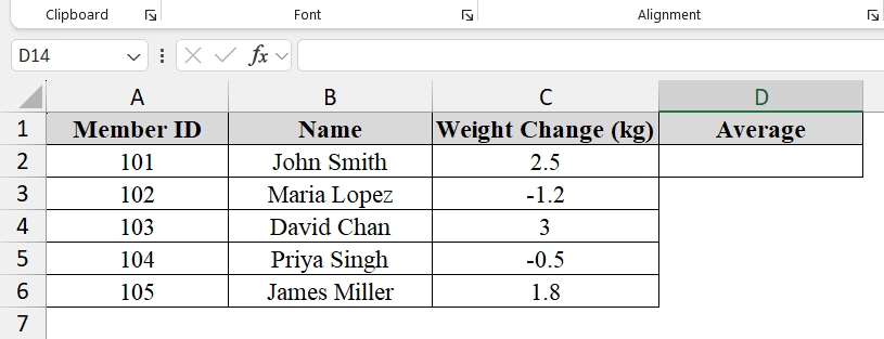
➤ Select the cell for your result and type the following formula in cell D2.
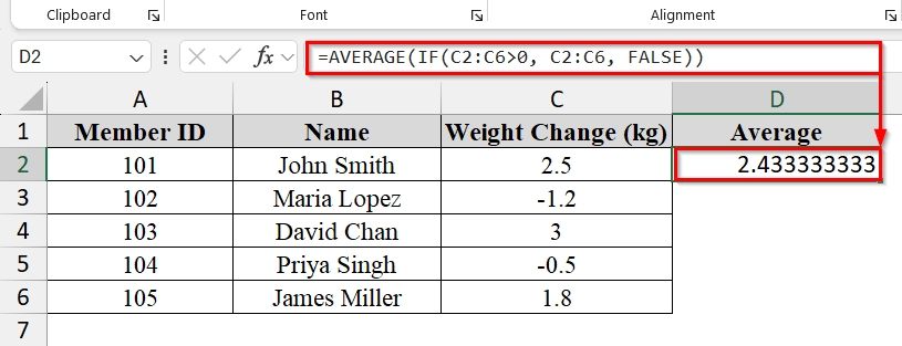
=AVERAGE(IF(C2:C6>0, C2:C6, FALSE))
➥ C2:C6 is the range of numbers we want to average.
➥ FALSE is used for values that do not meet the condition (ignored in calculation).
➤ If using Excel 2016 or earlier, press Ctrl + Shift + Enter instead of just Enter . Excel will automatically place curly braces {} around the formula. If using Excel 365 or Excel 2021, pressing Enter will work normally (Excel now handles arrays automatically).
Note:
➥ The formula ignores negative numbers and zeros.
➥ You can change the range (C5:C14) to fit your dataset.
➥ In modern Excel, no special key combination is needed for array formulas, just press Enter.
Frequently Asked Questions
Do I still need Ctrl + Shift + Enter in Excel 365?
No, modern Excel versions calculate arrays automatically without the CSE shortcut.
Can array formulas slow down my spreadsheet?
Yes, large arrays can impact performance if used in thousands of cells.
What is an example of a simple array formula?
=SUM(A1:A5*B1:B5) calculates the sum of products between two ranges.
Concluding Words
Excel array formulas allow us to process large data sets with minimal manual work. The practice file we used in the article can be downloaded for your exercise. Feel free to leave a comment to let us know your thoughts.