In a basic INDEX-MATCH formula, MATCH finds the position of a specific lookup value and INDEX uses that position number to fetch the value from a specific range. Although INDEX-MATCH is a powerful lookup tool, it has limitations such as not returning multiple values, finding the lowest number, returning customized texts, etc.
Adding the IF function allows for such customizations as it performs logical tests and returns different values based on whether a condition is met.
Steps to combine IF with INDEX-MATCH for getting different values for different conditions:
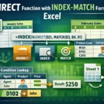
➤ First, we’ll put one of our lookup values (T101 or L101) in F2. If the value is T101, we want the formula to return the corresponding value from Column B. For L101, it should return the corresponding value from Column D.
➤ To achieve this, enter this formula in G2:
=IF(F2=”T101″, INDEX(B:B, MATCH(F2, A:A, 0)), IF(F2=”L101″, INDEX(D:D, MATCH(F2, A:A, 0)), “Code Not Found”))
➤ Change the lookup values T101 and L101, lookup range A:A, and result ranges B:B and D:D as needed. Press Enter.
In this article, we’ll cover more ways of combining the IF function with INDEX-MATCH for flexible conditional lookups, handling errors, returning customized texts, finding the highest or lowest numeric value, etc.
Basic Lookup with Dynamic Criteria
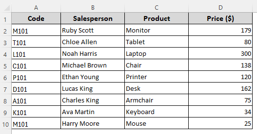
For visual aid, we’ll use the following sample dataset containing columns for some product codes, salesperson names, product names, and their prices.
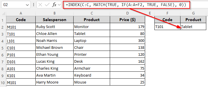
Adding the IF function allows for logical tests, so you can use it for complex lookups based on one or multiple conditions. In this basic method, we’ll set up a single criterion and find the first match based on it. We’ll look for the code T101 in Column A and return the product name for that code from Column C. Below are the details:
➤ Let’s enter the lookup value in F2 and insert this formula in G2 where we want to return the match:
=INDEX(C:C, MATCH(TRUE, IF(A:A=F2, TRUE, FALSE), 0))
➤ Change the lookup range A:A, return range C:C, and lookup cell reference F2 according to your dataset.
➤ Press Enter for Excel 365/2021. If you’re using an older version, use the Ctrl + Shift + Enter key.
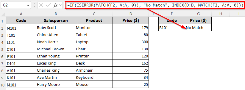
Replace Errors with Customized Texts
One major drawback of the INDEX-MATCH formula is that it returns #N/A when no match is found. To avoid #N/A and all types of errors and replace them with blanks or customized texts, we can use IF with ISERROR for Excel versions before 2007. For newer versions, you can use IFERROR instead. Below are the details:
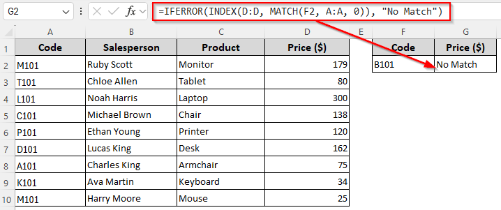
➤ Enter the lookup value B101 in F2 so that our formula can return the corresponding price for the code from Column D. If the value isn’t found, the following formulas will return a No Match customized text:
For Excel 2007 or Prior Versions
=IF(ISERROR(MATCH(F2, A:A, 0)), "No Match", INDEX(D:D, MATCH(F2, A:A, 0)))
➤ Replace the cell reference F2 containing the lookup value, lookup range A:A, and return range B:B according to your dataset. To return blanks, use “” instead of “No Match”. You can use any other customized texts.
➤ Press Enter.
For Versions After Excel 2007
=IFERROR(INDEX(D:D, MATCH(F2, A:A, 0)), "No Match")
➤ Change the lookup cell reference, lookup range, and return range as needed.
➤ Click Enter.
Return Customized Texts for Conditional Lookups
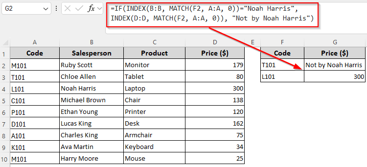
Use this method when you want to perform a lookup, but only if a certain condition is met. With the IF function, the INDEX-MATCH formula can return a customized text when the condition isn’t met. Here, our formula will return the price from Column D only if products T101 and L101 were sold by a specific salesperson Noah Harris.
If either of them was sold by someone else, the formula will return Not by Noah Harris instead of an error or blank.
➤ Enter the values T101 and L101 in F2 and F3. Insert the following formula in G2:
=IF(INDEX(B:B, MATCH(F2, A:A, 0))="Noah Harris", INDEX(D:D, MATCH(F2, A:A, 0)), "Not by Noah Harris")
➤ Change the lookup range A:A, lookup cell reference F2, and return ranges B:B and D:D as required. You can also change the texts.
➤ Press Enter and drag the formula down to G3 using the fill handle (+ sign on the bottom corner of the cell).
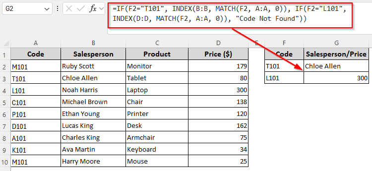
Return Different Values from Different Columns for Dynamic Conditions
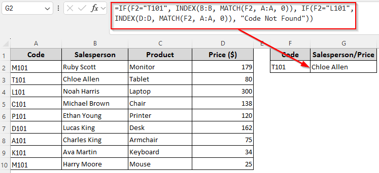
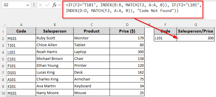
If you want different results from different columns depending on the lookup value, you can use the IF function to specify the conditions. Here, our lookup values are T101 and L101. When Excel finds T101 in the lookup range, we want it to return the corresponding salesperson’s name from Column B. For L101, it should return the product price from Column D. Let’s get to the steps:
➤ Enter the lookup value T101 in F2 and type the following formula in G2:
=IF(F2="T101", INDEX(B:B, MATCH(F2, A:A, 0)), IF(F2="L101", INDEX(D:D, MATCH(F2, A:A, 0)), "Code Not Found"))
➤ Replace the lookup values T101 and L101, lookup cell reference F2, lookup range A:A, and return ranges B:B and D:D depending on your source data.
➤ Press Enter and Excel will return the correct name for T101.
➤ When we enter L101, it returns the price as shown below:
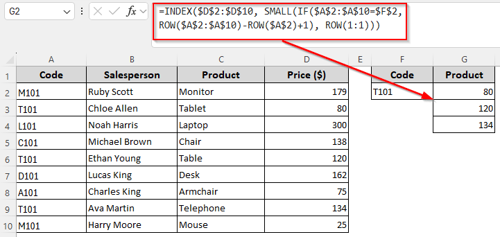
Extract All the Matches for a Lookup Value
As IF only performs logical tests, we’ll need the ROW function to generate sequential numbers and the SMALL function to find the smallest positions based on the results of the IF function. To find all the prices for the code T101, follow these steps:
➤ Enter the lookup value T101 in cell F2 and insert the following formula in cell G2:
=INDEX($D$2:$D$10, SMALL(IF($A$2:$A$10=$F$2, ROW($A$2:$A$10)-ROW($A$2)+1), ROW(1:1)))
➤ In this formula, adjust the lookup cell reference $F$2, first cell of the lookup range $A$2, lookup range $A$2:$A$10, and return range $D$2:$D$10 as per your source data.
➤ For Excel 365 and 2021, click Enter . If you’re using an older version, press Ctrl + Shift + Enter .
➤ Drag the formula down to return all the matches.
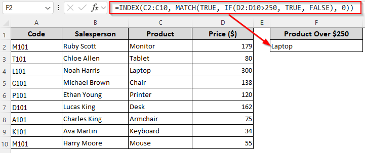
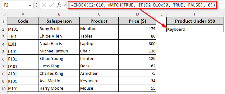
Conditional Lookup Based on Numeric Criteria
With the IF function, you can specify conditions with numeric values. We can use it to extract data when the value is lower or greater than a number you specify.
To find the first product with a price greater than 250 or lower than 50, follow the steps given below:
For Price Greater Than 250
➤ In a cell where you want to return the product name, insert this formula:
=INDEX(C2:C10, MATCH(TRUE, IF(D2:D10>250, TRUE, FALSE), 0))
➤ Here, D2:D10 is the lookup range and C2:C10, is the return range. Change these values as needed.
➤ Click Enter for Excel 365/2021. Use Ctrl + Shift + Enter for older Excel versions.
For Price Lower Than 50
➤ Enter this formula to return the correct product:
=INDEX(C2:C10, MATCH(TRUE, IF(D2:D10<50, TRUE, FALSE), 0))
➤ Replace the lookup and return ranges as required.
➤ Press Enter or Ctrl + Shift + Enter depending on your Excel version.
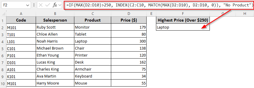
Find the Highest/Lowest Numeric Value Based on Numeric Criteria
This time we’ll specify numeric conditions to return results based on the highest or lowest value matching that condition. For example, our formula will check if the highest/lowest value in Column D is higher than 250/lower than 50. If yes, it returns the corresponding value from Column C. If no, the formula returns a No Product customized text. Below are the details:
For the Highest Price Which Is Higher Than 250
If you want to find the product with the highest price, and only return it if it’s higher than 250, enter this formula:
=IF(MAX(D2:D10)>250, INDEX(C2:C10, MATCH(MAX(D2:D10), D2:D10, 0)), "No Product")
➤ To match your source data, change the lookup range C2:C10, return range D2:D10, and numeric condition as needed.
➤ Press Enter.
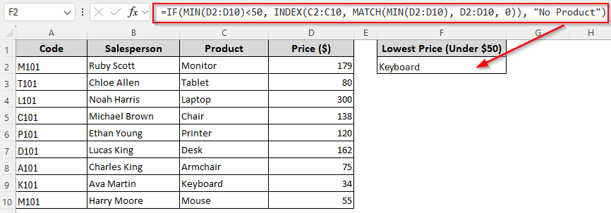
For the Lowest Price Which Is Lower Than 50
➤ Use this formula if you want to find the product with the lowest price and only return the product name if the price is below 50:
=IF(MIN(D2:D10)<50, INDEX(C2:C10, MATCH(MIN(D2:D10), D2:D10, 0)), "No Product")
➤ Replace the ranges and conditions as required.
➤ Click Enter.
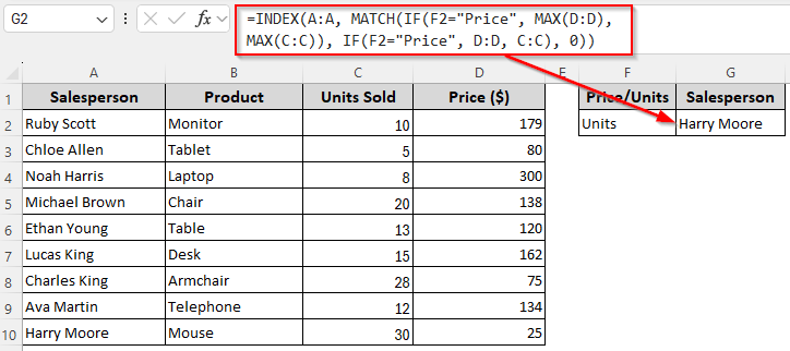
Find Match Based on the Highest/Lowest Numeric Value from Different Ranges
For this method, we’ll remove the column for product codes and add a new column containing the number of units sold. We’ll use a formula with IF and INDEX-MATCH to find the value corresponding to the highest or lowest numeric value from these two ranges.
If we insert Price in F2, the formula should return the salesperson’s name with the highest/lowest product price. When we insert Units, it will give the salesperson’s name who sold the highest/lowest number of units. Here are the steps:
➤ In cell F2, insert the lookup value Price or Units. Now, enter any of the following formulas in G2:
Find the Salesperson’s Name for the Highest Value
➤ Use this formula to get the salesperson’s name who sold the product with the highest price:
=INDEX(A:A, MATCH(IF(F2="Price", MAX(D:D), MAX(C:C)), IF(F2="Price", D:D, C:C), 0))
➤ Change the lookup ranges C:C and D:D, lookup cell reference F2, and return range D:D according to your dataset.
➤ Depending on your Excel version, use Enter or Ctrl + Shift + Enter .
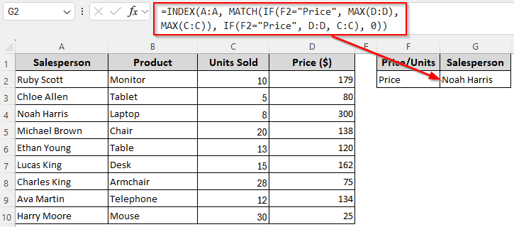
➤ To get the salesperson’s name who sold the most number of units, enter Units in F2 and the result will change automatically.
Find the Salesperson’s Name for the Lowest Value
➤ Insert this formula to extract the salesperson’s name corresponding to the lowest product price:
=INDEX(A:A, MATCH(IF(F2="Price", MIN(D:D), MIN(C:C)), IF(F2="Price", D:D, C:C), 0))
➤ Change the lookup and return ranges as per your source data.
➤ Click Enter or Ctrl + Shift + Enter based on your Excel version.
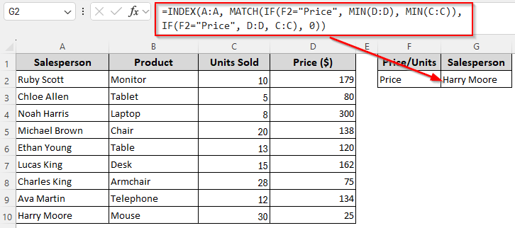
➤ To get the result for the lowest number of units, enter Units in F2.

Frequently Asked Questions
Can you use IF and MATCH together in Excel?
Yes. You can wrap MATCH inside an IF statement to create conditional lookups. For example, use the following formula to find the row number of the product with the minimum price only if it is below 100:
=IF(MIN(D:D)<100, MATCH(MIN(D:D), D:D, 0), “No Match”)
Change the lookup range D:D and the numeric condition to match your source data. Press Enter. If no match is found, the formula returns No Match.
How do you write 3 conditions with the IF function in Excel?
You can nest multiple IF statements to handle more than one condition. To give an example, we’ll categorize the product prices in Column D into three groups. For prices below 150, the formula will return Low. Prices between 150 and 250 are in the Medium category and prices above 250 will be categorized as High. Here’s the formula:
=IF(D2<150,”Low”, IF(D2<=250,”Medium”,”High”))
Change the first cell of the source range D2 and the prices according to your dataset and click Enter.
Can I combine IFS and INDEX-MATCH?
Yes, you can use IFS to control which column or criteria to use and then pair it with INDEX-MATCH to return the corresponding value. Let’s say F2 contains Price or Units and we want the salesperson who achieved the highest value from Column C (units) or Column D (price) based on the value in F2. For this, we’ll use the following formula:
=IFS(F2=”Price”, INDEX(B:B, MATCH(MAX(D:D), D:D, 0)), F2=”Units”, INDEX(B:B, MATCH(MAX(C:C), C:C, 0)), TRUE, “Invalid Criteria”)
Replace the lookup ranges C:C and D:D, return range B:B, and lookup cell reference F2 as required. Press Enter. If F2 contains anything other than Price or Units, the formula returns Invalid Criteria.
Concluding Words
Depending on what condition you want, you can combine or nest the IF function with INDEX-MATCH in many different ways. For added flexibility, you can include more functions like AND, OR, MAX, MIN, ROW, and SMALL in conditional lookups. Instead of IF, you can also use IFNA, IFS, IFERROR to handle errors and conditions with a simpler formula syntax.