In a typical INDEX-MATCH formula, MATCH finds the row/column number of a value and INDEX returns the value at that position. The SUMPRODUCT function is used to sum values that meet conditions. Combining the three functions allows you to perform aggregate calculations based on multiple, dynamic conditions.
Usually, they are used to find a row based on one criterion and a column based on another. You can also use them to find multiple rows and columns based on multiple conditions.
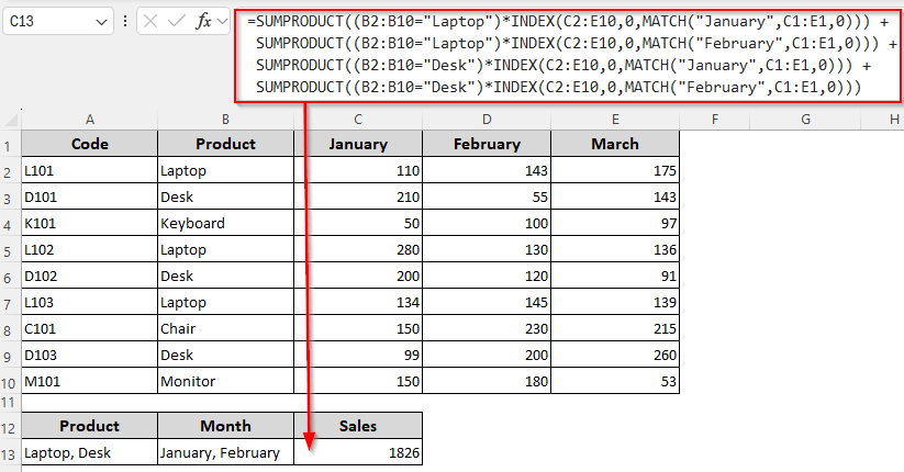
➤ In a dataset with product names and their monthly sales across 3 columns, we’ll look for the values Laptop and Desk and sum their sales for January and February. For this, we’ll use the following formula:
=SUMPRODUCT((B2:B10=”Laptop”)*INDEX(C2:E10,0,MATCH(“January”,C1:E1,0)))+SUMPRODUCT((B2:B10=”Laptop”)*INDEX(C2:E10,0,MATCH(“February”,C1:E1,0)))+SUMPRODUCT((B2:B10=”Desk”)*INDEX(C2:E10,0,MATCH(“January”,C1:E1,0)))+SUMPRODUCT((B2:B10=”Desk”)*INDEX(C2:E10,0,MATCH(“February”,C1:E1,0)))
➤ Change the row criteria Laptop and Desk along with their lookup range B2:B10 according to your dataset. You also need to replace the column criteria for January and February, along with their lookup range C1:E1.
➤ Press Enter for Excel 365/2021 or Ctrl + Shift + Enter for older versions.
This article covers all the ways of combining SUMPRODUCT with INDEX-MATCH based on a single or multiple criteria, numeric conditions, etc.
Summation Based on a Single Row and Column Criterion
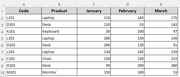
For visual demonstration, we have a sample dataset with columns for product codes (Column A), names (Column B), and monthly sales figures for January (Column C), February (Column D), and March (Column E). We’ll calculate the sales sum of one or multiple months (column criteria) for one or multiple products (row criteria).
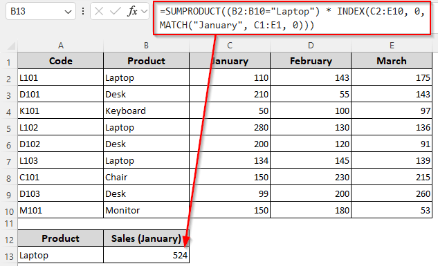
To calculate the sales sum of January for Laptop, use any of the following formulas:
Formula with Lookup Texts
➤ Here, we’ll insert our lookup texts Laptop and January directly in the following formula:
=SUMPRODUCT((B2:B10="Laptop")*INDEX(C2:E10,0,MATCH("January",C1:E1,0)))
➤ Depending on your source data, replace the row criteria Laptop and its lookup range B2:B10, column criteria January and its lookup range C1:E1, and return range C2:E10 containing the values to sum.
➤ For Excel 365/2021, click Enter . Press Ctrl + Shift + Enter for older versions.
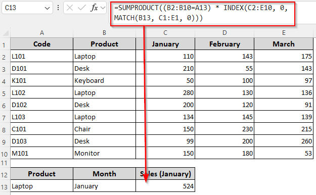
Formula with Cell References
➤ If the lookup values are in A13=Laptop and B13=January, enter the following formula in a cell where you want the summed value:
=SUMPRODUCT((B2:B10=A13) * INDEX(C2:E10, 0, MATCH(B13, C1:E1, 0)))
➤ Change the cell references and ranges according to your dataset.
➤ Press Enter or Ctrl + Shift + Enter depending on your Excel version.
Extract Sum Based on One or Two Row and Column Criteria
Now, we’ll find the sales sum of one or two months (column criteria) for one or two products (row criteria). Depending on your criteria, use any of the following formulas:
1 Row, 2 Columns Criteria
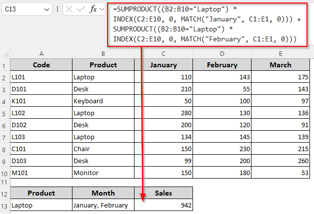
Find Laptop’s sales for January and February with the following formula:
=SUMPRODUCT((B2:B10="Laptop")*INDEX(C2:E10,0,MATCH("January",C1:E1,0)))+SUMPRODUCT((B2:B10="Laptop")*INDEX(C2:E10,0,MATCH("February",C1:E1,0)))
➤ Based on your source data, replace the row criteria Laptop and its lookup range B2:B10, column criteria January, February and their lookup range C1:E1, and return range C2:E10 containing the sales figures to sum.
➤ Press Enter for Excel 365/2021. If you’re using an older version, click Ctrl + Shift + Enter on your keyboard.
2 Rows, 1 Column Criteria
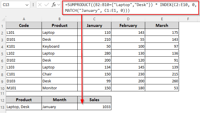
Sum the sales figures for Laptop and Desk in January using this formula:
=SUMPRODUCT((B2:B10={"Laptop","Desk"})*INDEX(C2:E10,0,MATCH("January",C1:E1,0)))
➤ Replace the lookup values and ranges as needed.
➤ Depending on your Excel version, press Enter or Ctrl + Shift + Enter .
2 Rows, 2 Columns Criteria
Insert the formula given below to find Laptop and Desk sales for January and February:
=SUMPRODUCT((B2:B10="Laptop")*INDEX(C2:E10,0,MATCH("January",C1:E1,0)))+SUMPRODUCT((B2:B10="Laptop")*INDEX(C2:E10,0,MATCH("February",C1:E1,0)))+SUMPRODUCT((B2:B10="Desk")*INDEX(C2:E10,0,MATCH("January",C1:E1,0)))+SUMPRODUCT((B2:B10="Desk")*INDEX(C2:E10,0,MATCH("February",C1:E1,0)))
➤ To match your source data, change the values and cell references.
➤ Use Enter or Ctrl + Shift + Enter depending on your Excel version.

Calculate Sum Depending on One/Two/All Row and Column Criteria
In this section, we’ll find the sales sum for all months for one or two products. Our formulas will also cover the summed value for all products in one or two months. Based on the outcome you want, choose any of the following formulas:
1 Row, All Columns Criteria
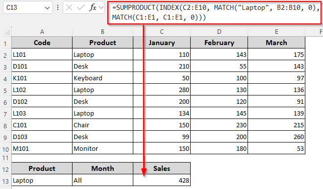
Find Laptop’s sales across all months with this formula:
=SUMPRODUCT(INDEX(C2:E10,MATCH("Laptop",B2:B10,0),MATCH(C1:E1,C1:E1,0)))
➤ Change the row criteria Laptop and its lookup range B2:B10, lookup range for column criteria C1:E1, and return range C2:E10 with the sales figure according to your dataset.
➤ Press Enter.
2 Rows, All Columns Criteria
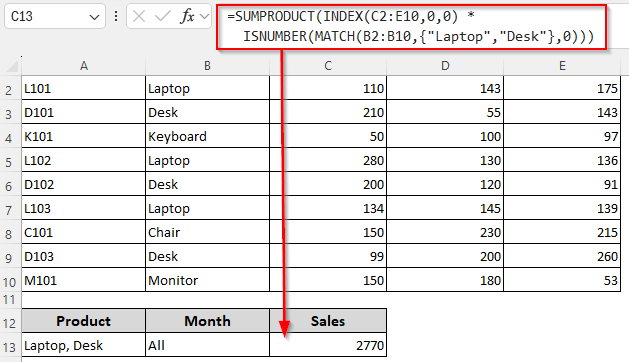
Sum the sales for Laptop and Desk across all months using the following formula:
=SUMPRODUCT(INDEX(C2:E10,0,0)*ISNUMBER(MATCH(B2:B10,{"Laptop","Desk"},0)))
➤ Replace the criteria and ranges according to your dataset.
➤ Use Enter or Ctrl + Shift + Enter based on your Excel version.
All Rows, 1 Column Criteria
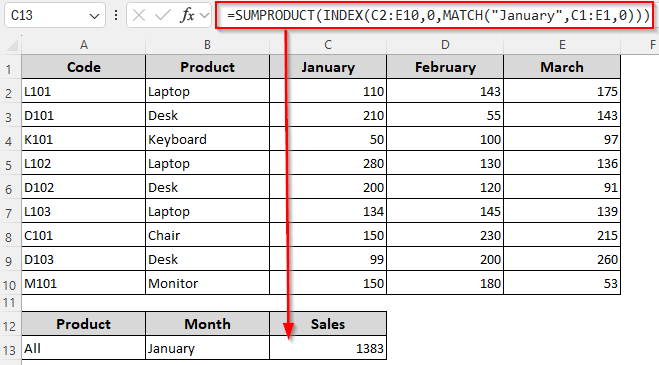
To get all product sales for January, apply this formula:
=SUMPRODUCT(INDEX(C2:E10,0,MATCH("January",C1:E1,0)))
➤ Here, all our products (row criteria) are in the range B2:B10. Column criteria January is in C1:E1 and the sales figures to sum are in C2:E10. Change these values based on your source data.
➤ Click Enter.
All Rows, 2 Columns Criteria
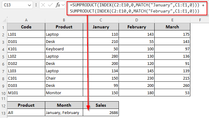
Here’s the formula to extract all product sales for January and February:
=SUMPRODUCT(INDEX(C2:E10,0,MATCH("January",C1:E1,0)))+SUMPRODUCT(INDEX(C2:E10,0,MATCH("February",C1:E1,0)))
➤ Depending on your dataset, replace the values and ranges as needed.
➤ Press Enter.
Determine the Sum with Product-Month Pairs
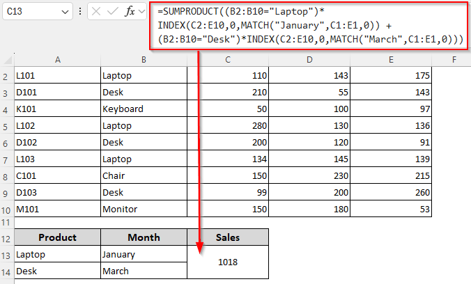
Now, we’ll calculate the sales sum of Laptop in January along with the sales sum of Desk in March. Here’s how to do it using a single formula:
Formula with Lookup Texts
=SUMPRODUCT((B2:B10="Laptop")*INDEX(C2:E10,0,MATCH("January",C1:E1,0))+(B2:B10="Desk")*INDEX(C2:E10,0,MATCH("March",C1:E1,0)))
➤ Here, our lookup values Laptop and Desk are in B2:B10. The second pair of lookup values, January and March, is in C1:E1. The sales value to sum is in C2:E10. Change the values and ranges to match your dataset.
➤ Click Enter.
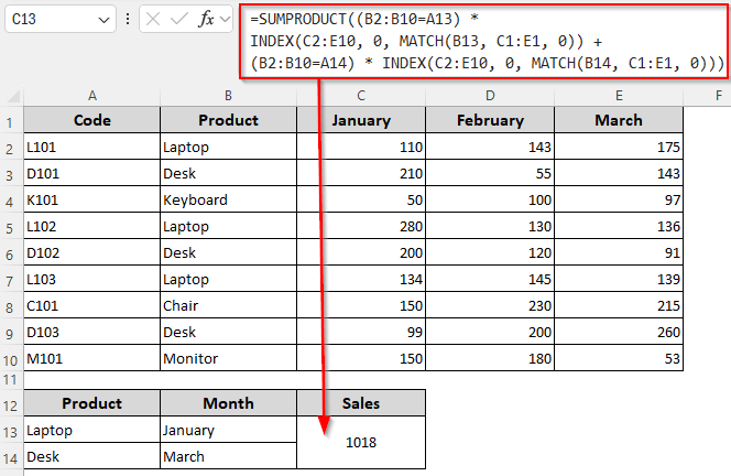
Formula with Cell References
Let’s say A13 contains the product name Laptop and B13 contains January. Similarly, A14=Desk and B14=March. We’ll use this formula to calculate the sum:
=SUMPRODUCT((B2:B10=A13) * INDEX(C2:E10, 0, MATCH(B13, C1:E1, 0)) + (B2:B10=A14) * INDEX(C2:E10, 0, MATCH(B14, C1:E1, 0)))
➤ Change the cell references and related ranges as required.
➤ Press Enter.
Calculate Sum Based on Numeric Condition
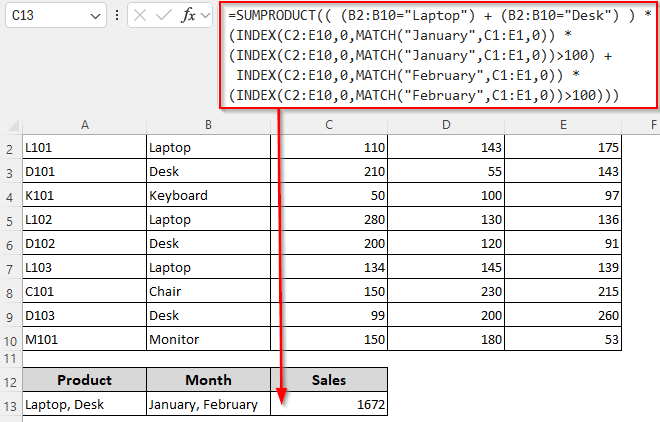
Now, let’s calculate the sum for the products Laptop and Desk in January and February only if the sales figure is over 100. Below are the steps:
➤ Select a cell where you want the output and enter this formula:
=SUMPRODUCT(((B2:B10="Laptop")+(B2:B10="Desk"))*(INDEX(C2:E10,0,MATCH("January",C1:E1,0))*(INDEX(C2:E10,0,MATCH("January",C1:E1,0))>100)+INDEX(C2:E10,0,MATCH("February",C1:E1,0))* (INDEX(C2:E10,0,MATCH("February",C1:E1,0))>100)))
➤ Change the lookup values Laptop, Desk, and their lookup range B2:B10. Replace the months January, February, and their lookup range C1:E1. Finally, adjust the return range C2:E10 and numeric condition >100 if needed.
➤ Click Enter.
Frequently Asked Questions
Can I Use SUMPRODUCT and XLOOKUPUP together?
Yes, you can use XLOOKUP with SUMPRODUCT to fetch arrays and then sum the values based on the specified condition(s). To calculate the total sales for Laptop and Desk in January and February, we’ll use this formula:
=SUMPRODUCT(XLOOKUP({"Laptop","Desk"}, B2:B10, C2:C10) + XLOOKUP({"Laptop","Desk"}, B2:B10, D2:D10))
Change the lookup values, their lookup ranges, and the return range as required. Press Enter.
How to find the largest sum with SUMPRODUCT and INDEX-MATCH?
To find the largest monthly sale for Laptop across January to March, use the following formula:
=SUMPRODUCT(MAX(INDEX(C2:E10, MATCH("Laptop", B2:B10, 0), 0)))
Replace the lookup values and ranges to match your source data and press Enter.
How to use SUMPRODUCT and INDEX-MATCH for weighted average?
Let’s say we have Column B=Product, Column C=Sales, and Column D=Weight (e.g., % contribution, rating, or importance). To calculate the weighted average for Laptop and Desk, use this formula:
=SUMPRODUCT(( (B2:B10="Laptop") + (B2:B10="Desk") ) * C2:C10 * D2:D10) / SUMPRODUCT(( (B2:B10="Laptop") + (B2:B10="Desk") ) * D2:D10)
Replace the ranges and values as needed and click Enter.
Concluding Words
While using SUMPRODUCT, remember that it treats TRUE as 1 and FALSE as 0. So, using multiplication (*) acts as an AND operator, while addition (+) acts as an OR operator.
Also, when combining these functions, locking your ranges with $ (e.g., $A$1:$A$100) is crucial to prevent errors when copying formulas. Otherwise, the formulas will return a #REF error when you copy the formula into a different range.