Return Multiple Values Vertically with INDEX-MATCH in Excel

Excel’s MATCH function finds the position (row or column number) of your lookup value. INDEX goes to that position in a different range and returns the value found there. By default, the INDEX-MATCH formula can’t return multiple matches.

However, combining them with other functions like SMALL, IF, and ROW allows you to get all the matches vertically in a list based on one or multiple criteria. To avoid errors when no more matches are found, we’ll wrap the formula with IFERROR.

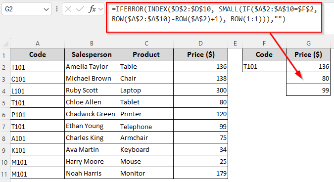
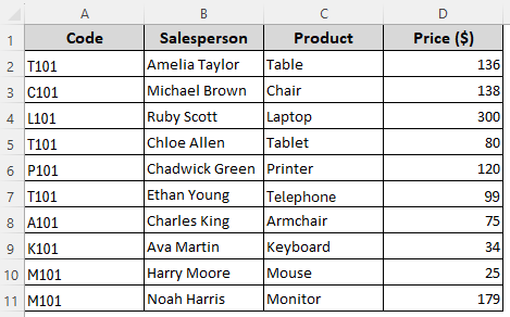
In our sample dataset, we have some product codes, salespeople’s names, product names, and product prices in columns A, B, C, and D. The code T101 is in the cells A2, A5, and A7. Our goal is to find all the prices for that code ($136, $80, and $99) from Column D.

In this method, the IF function checks each value in the lookup range and returns the row positions where the condition is true. SMALL picks the nth smallest position from the IF results, based on the current row number. ROW generates a sequential number (1, 2, 3, …) as you copy the formula downward. Finally, IFERROR replaces errors with a blank. Here’s how to use them together:

➤ First, we’ll enter the code T101 in cell F2 to use it as a reference for our formula. As we want to put the first returned match in cell G2, we’ll insert the following formula in G2:

➤ Here, $A$2:$A$10 is our lookup range containing the values we’re looking for and $D$2:$D$10 is the return range from where we’ll get the matched results. $F$2 contains the lookup value and $A$2 is the first cell of the lookup range. Replace these values with references from your source data.
➤ If you’re using an Excel version before Excel 365/2021, press  Ctrl  +  Shift  +  Enter  . For newer versions, click  Enter  . Use the fill handle (+ sign on the bottom corner of the cell) to drag the formula until it returns a blank.

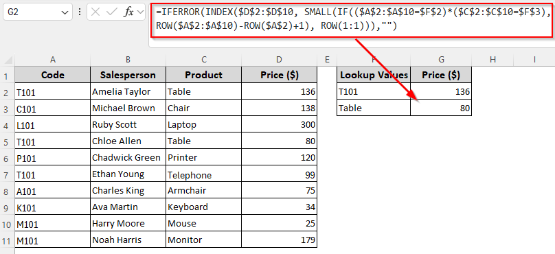
In this method, we’ll set two different conditions and use a formula to return all the matches meeting both conditions. Here, we’ll extract the prices based on the product code and name.

So, we’ll insert the product code (1st criterion) in F2 and the product name (2nd criterion) in F3. Let’s get to the steps:

➤ In cell G2, where we want to return the first match, type the following formula:

➤ Here, cells $F$2 and $F$3 contain the lookup values. $A$2:$A$10 and $C$2:$C$10 are the lookup ranges. $A$2 is the first cell of our range and $D$2:$D$10 is the return range. Change the references as required.
➤ Use  Enter  or  Ctrl  +  Shift  +  Enter  based on your Excel version. Drag the formula down until it returns blanks.

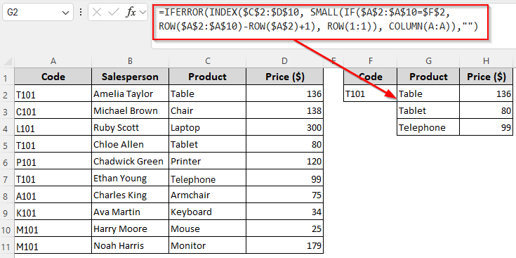
Use this method to get multiple results from two different columns based on a single criterion. Here, we’ll extract the product names in Column G and their prices in Column H for the lookup value T101. Here’s how:

➤ First, enter the lookup value in F2. In cell G2 where you want the first match from the first column, insert this formula:

➤ Replace the lookup range $A$2:$A$10, return range C$2:$D$10, and lookup cell reference $F$2 as needed.
➤ Based on your Excel version, click  Enter  or  Ctrl  +  Shift  +  Enter  .
➤ Drag the formula down and then across to get all the matches from columns C and D into columns G and H.

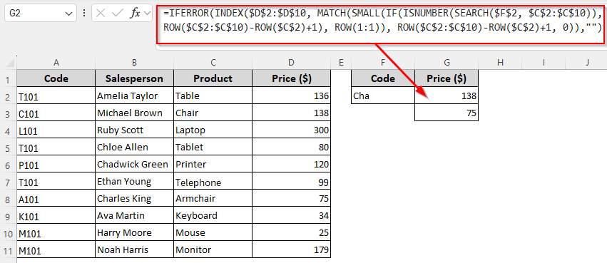
While the SEARCH function returns positions where the lookup value is found, ISNUMBER returns TRUE/FALSE for matches so that IF can work on the matches only (ignoring FALSE). In this example, we’ll look for the value Cha in the product name column (Column C). Excel will return the prices from Column D for all products partially matching the lookup value (Chair and Armchair). Below is the process:

➤ Put the lookup value Cha in column F2 and enter this formula in G2:

➤ Change the lookup range $C$2:$C$10, first cell of the lookup range $C$2, return range $D$2:$D$10, and lookup cell reference $F$2 as per your source data.
➤ Press  Enter  or  Ctrl  +  Shift  +  Enter  depending on your Excel version.
➤ Drag the formula down to get all matches.

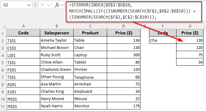
Here, we want to look into Column B and Column C for any values partially matching Cha. Our formula returns the prices from Column D for all the matches from both columns. Let’s get to the steps:

➤ Enter the lookup value Cha in F2 and insert this formula in G2:

➤ To match your source data, change the lookup ranges B$2:$B$10 and C$2:$C$10, lookup cell reference $F$2, return range D$2:$D$10, and first cell of the return range $D$2 as needed.
➤ Press  Enter  or  Ctrl  +  Shift  +  Enter  based on your Excel version.
➤ Drag the formula down until you get blanks.

Frequently Asked Questions

What can I use instead of INDEX-MATCH for multiple matches?

You can use FILTER (Excel 365/2021) to instantly return all matches at once, or use INDEX + SMALL + IF in older Excel versions. If your lookup value is in F2, the lookup range is A2:A10, and the return range is D2:D10, use any of the following formulas:
=FILTER($D$2:$D$10, $A$2:$A$10=$F$2, “No Match”)
Or,
=IFERROR(INDEX($D$2:$D$10, SMALL(IF($A$2:$A$10=$F$2, ROW($A$2:$A$10)-ROW($A$2)+1), ROW(1:1))),””)
Press  Enter  for the first formula and  Ctrl  +  Shift  +  Enter  for the second one ( when used in older Excel). Drag the formula for all matches.

How to return multiple results with INDEX-MATCH without duplicates?

Yes, you can use INDEX-MATCH to return multiple results by combining the COUNTIF function. If your lookup range is A2:A10, return range is D2:D10, lookup value is in F2, and the return column starts in G2, enter this formula in G2:
=IFERROR(INDEX($D$2:$D$10, MATCH(1, (COUNTIF($G$1:G1, $D$2:$D$10)=0) * ($A$2:$A$10=$F$2), 0)),””)
Change the references as needed. Press  Enter  or  Ctrl  +  Shift  +  Enter  depending on your Excel version and drag the formula down.

Can INDEX-XMATCH return multiple values?

By default, the INDEX-XMATCH formula returns only the first match. But we can combine it with SEQUENCE, ROW, IF, and ROWS to get multiple matches. Here’s the formula:
=INDEX($D$2:$D$10, XMATCH(SEQUENCE(ROWS($A$2:$A$10)), IF($A$2:$A$10=$F$2, ROW($A$2:$A$10)-ROW($A$2)+1)))
You need to change the lookup cell reference $F$2, lookup range $A$2:$A$10, and the return range is $D$2:$D$10 according to your dataset. Use  Enter  or  Ctrl  +  Shift  +  Enter  based on your Excel version. Drag the formula down to get multiple results.

Concluding Words

If you’re using an older version of Excel, the INDEX-MATCH-SMALL-IF array formula is the best solution for complex lookups. However, in newer versions, the FILTER function solves the multiple-match issue with its simple syntax. You can also use XLOOKUP to handle multiple results easily, especially with dynamic arrays.