Advanced Excel
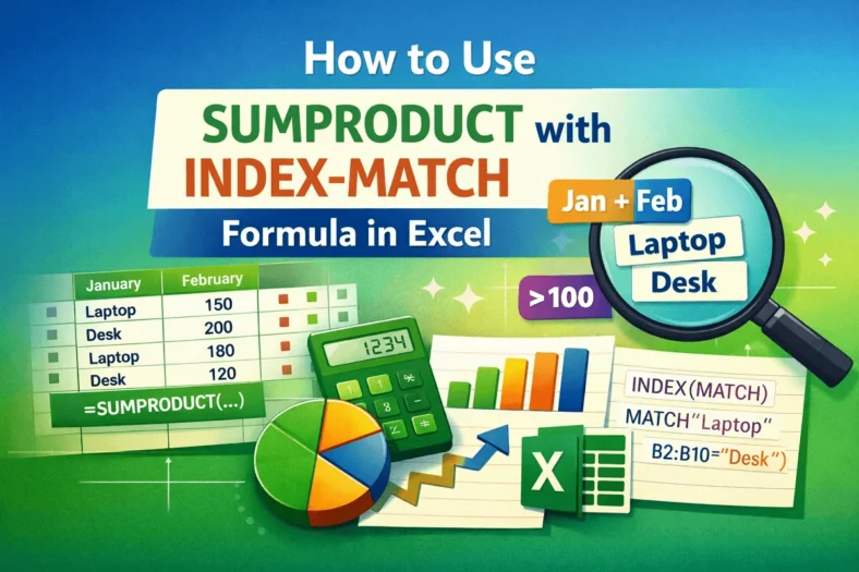
How to Use SUMPRODUCT with INDEX-MATCH Formula in Excel
In a typical INDEX-MATCH formula, MATCH finds the row/column number of a value and INDEX returns the value at that position. The SUMPRODUCT function is used to sum values that


In a typical INDEX-MATCH formula, MATCH finds the row/column number of a value and INDEX returns the value at that position. The SUMPRODUCT function is used to sum values that
With Excel’s Conditional Formatting feature, you can apply formatting (e.g., color fills, font changes, or borders) to cells based on specific rules. Excel’s built-in Text That Contains option only works
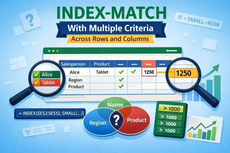
A simple INDEX-MATCH formula handles single criteria, but when you need to match both rows and columns with multiple criteria, you need more advanced formulas. By default, MATCH finds the
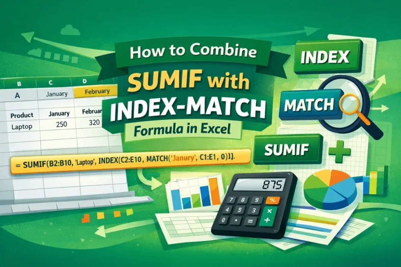
In the INDEX-MATCH formula, MATCH finds the relative position of a lookup value in a range and INDEX returns a match from a specified row and column in a range
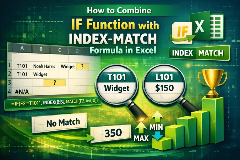
In a basic INDEX-MATCH formula, MATCH finds the position of a specific lookup value and INDEX uses that position number to fetch the value from a specific range. Although INDEX-MATCH
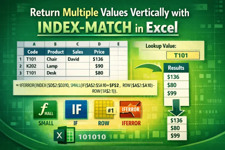
Excel’s MATCH function finds the position (row or column number) of your lookup value. INDEX goes to that position in a different range and returns the value found there. By
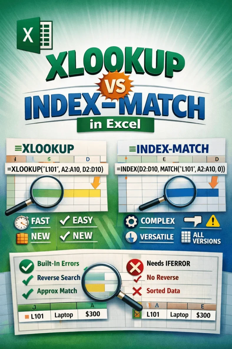
Both INDEX-MATCH and XLOOKUP are two powerful lookup functions in Excel used to find data from a specific range. You can use them for exact matches, approximate matches, two-way lookups,
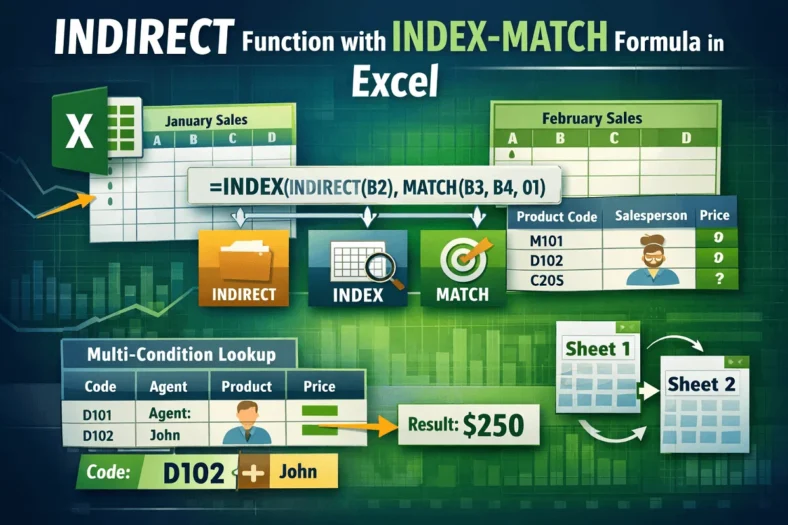
Excel’s MATCH function looks for a specific item in a row or column and tells you its position. While INDEX returns the value at a specific position in a range,
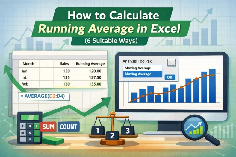
Calculating running averages for time-based data is best for long-term projects, sales analysis, and recognizing changing trends. Here, we take a certain period and calculate the average of our data.