The COUNTIFS function in Excel is an excellent tool that lets you count the number of entries that meet multiple criteria. But beyond the basic syntax, there are many advanced use cases that make it even more useful for real-world data analysis. Whether you’re working with date ranges, partial text matches, logical conditions, or structured tables, COUNTIFS can help simplify complex calculations.
In this article, we’ll learn the most practical and advanced ways to use the COUNTIFS function using named ranges for better formula clarity, filter data between dynamic date ranges using functions like TODAY and EOMONTH, handle partial matches and blanks with wildcards, simulate OR logic within COUNTIFS, and apply COUNTIFS inside Excel Tables to create dynamic and easy-to-update reports.
Steps to use the advanced COUNTIFS function in Excel:
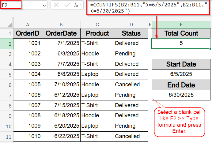
➤ Select a blank cell where you want the result, such as F2.
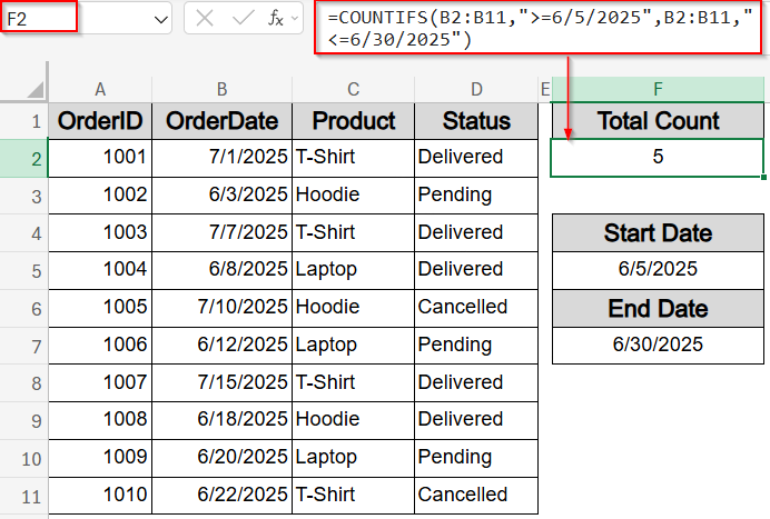
➤ To count orders between two fixed dates (e.g., June 5 to June 30), enter this formula:
=COUNTIFS(B2:B11,”>=6/5/2025″,B2:B11,”<=6/30/2025″)
Here, B2:B11 contains the order dates. The formula returns the number of rows with order dates between June 5 and June 30, 2025, inclusive.
➤ Press Enter to see the result.
Count Data Within a Dynamic Date Range and Specific Criteria
When analyzing orders, you may need to count how many orders were placed within a specific date range and have a certain status such as “Delivered“. In this method, we’ll demonstrate how to count orders between a custom date range and with a specific status like “Delivered” or “Pending.” We’ll also explore a dynamic alternative that uses the TODAY function to track recent activity automatically.
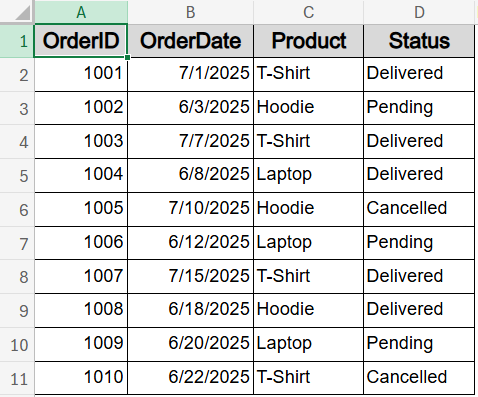
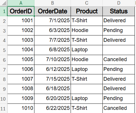
We’ll use a sample dataset that includes recent 2025 sales records with order IDs, order dates, product names, and delivery statuses for demonstrating real-world applications of advanced COUNTIFS techniques across text, dates, and conditions.
Steps:
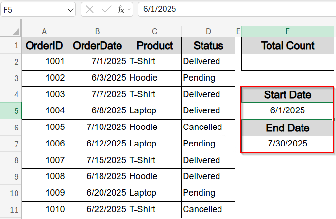
➤ Enter your custom start date in cell F5 (e.g., 2025-06-01) and end date in F7 (e.g., 2025-07-30).
➤ In a blank cell (e.g., H2), type the following formula to count orders between those dates with status “Delivered“:
=COUNTIFS(B2:B11, “>=”&F5, B2:B11, “<=”& F7, D2:D11, “Delivered”)
This counts all rows where the OrderDate (B2:B11) falls between the values in F5 and F7, and the Status column (D2:D11) is exactly “Delivered“.
➤ Press Enter to see the result.
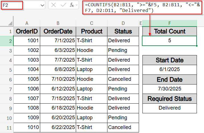
Now you’ll get the number of delivered orders placed within your custom range.
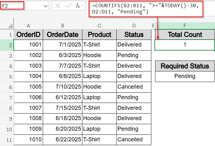
➤ Alternatively, use this dynamic formula in F2 cell to count recent orders that are still pending as of today:
=COUNTIFS(B2:B11, “>=”&TODAY()-30, D2:D11, “Delivered”)
This formula calculates the count of “Pending” orders placed within the last 30 days, based on today’s date.
➤ Press Enter and this value will auto-update daily without needing to adjust the date range manually.
This technique helps you monitor your order trends over time both in fixed and dynamic ranges using just one formula that adjusts dynamically.
Set Up Named Ranges to Use with COUNTIFS Function
COUNTIFS function is ideal when you need to apply multiple filters at once, for example, checking how many entries match a specific product name and a related status. You can simplify your formulas further by using named ranges instead of standard A1-style references, which improves readability and simplifies maintenance.
In this example, we’ll count how many times the Product is “T-Shirt” and the Status is “Delivered” in our dataset using named ranges.
Steps:
➤ Go to the Formulas tab >> Name Manager >> Define Name.
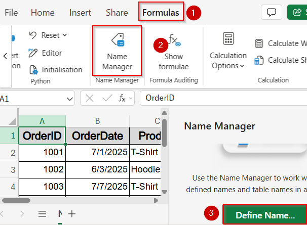
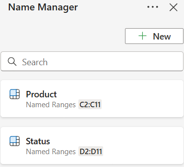
➤ Define range C2:C11 as Product and D2:D11 as Status.
➤ Click on any blank cell like F2.
➤ Type this formula:
=COUNTIFS(Product, “T-Shirt”, Status, “Delivered”)
➤ Press Enter.
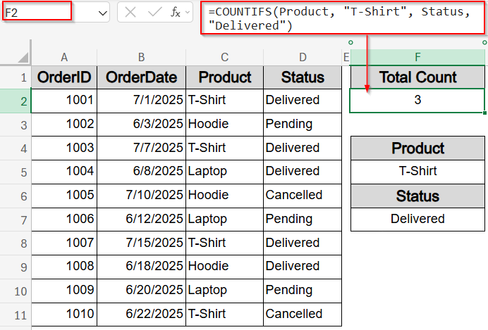
Now this references our defined ranges without hardcoding inside the formula for the chosen Product and Status.
COUNTIFS Function to Count Data Within a Specific Date Range
When analyzing orders by timeline, you might want to count how many were placed within a specific period or during a full calendar month. The COUNTIFS function lets you filter date-based entries precisely using greater than (>=), less than (<=) operators, and helper functions like EDATE.
In this method, we’ll count how many orders were placed during a selected date range, and also how many fall within the month of June 2025. These are especially useful when preparing time-based summaries or monthly reports.
Steps:
➤ Select a blank cell where you want the result, such as F2.
➤ To count orders between two fixed dates (e.g., June 5 to June 30), enter this formula:
=COUNTIFS(B2:B11,”>=6/5/2025″,B2:B11,”<=6/30/2025″)
Here, B2:B11 contains the order dates. The formula returns the number of rows with order dates between June 5 and June 30, 2025, inclusive.
➤ Press Enter to see the result.
Excel will return how many orders fall inside this custom range.
➤ Alternatively, type this formula in another cell to count how many orders were placed in June 2025 using a dynamic calendar filter:
=COUNTIFS(B2:B11,”>=”&DATE(2025,6,1),B2:B11,”<“&EDATE(DATE(2025,6,1),1))
This formula uses the DATE function to start at June 1, 2025, and the EDATE function to auto-calculate the end of the month. It counts all orders within that full calendar month.
➤ Press Enter again.
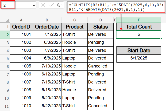
You’ll now have a count of all orders placed during June 2025 based on the date logic.
Use COUNTIFS Function for Partial Text Matches and Excluding Blanks
When working with real-world data, it’s common to encounter partial text values and occasional missing entries. The COUNTIFS function allows you to handle both scenarios using wildcards (* and ?) and logical operators like <> for “not equal to.” This technique is especially useful when preparing data for reporting, ensuring completeness, or pulling entries based on partial keywords.
In this method, we’ll count how many products contain a specific keyword (like “Shirt”) and also count how many rows have both a non-empty Product and Status to help clean up data or validate entries in your list. This is the modified dataset we will be using:
Steps:
➤ Click on a blank cell where you want the first result, such as F2.
➤ Enter the following formula to count all products that include the word “Shirt”:
=COUNTIFS(C2:C11, “*Shirt*”)
Here, C2:C11 refers to the Product column. The asterisk * acts as a wildcard to match any number of characters before or after “Shirt”.
➤ Press Enter to get the result.
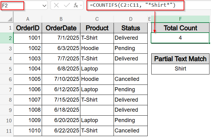
Excel will return the count of all rows where the product contains “Shirt,” such as “T-Shirt.”
➤ Now in another cell, enter this formula to count only rows where both Product and Status are filled in:
=COUNTIFS(C2:C11, “*”, D2:D11, “<>”)
This checks that the Product column is not blank and the Status column also has a value.
➤ Press Enter again.
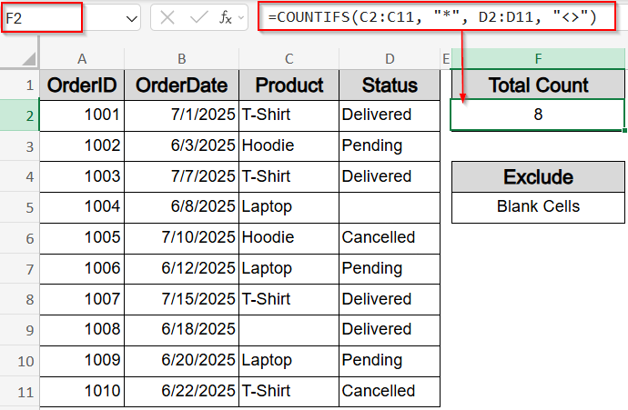
You’ll now see how many rows are fully filled out in those two fields.
Simulate OR Logic with COUNTIFS Function Using Arrays or Additions
The COUNTIFS function is designed to apply multiple conditions using AND logic, but there are times when you need to count values that meet one condition or another. While COUNTIFS doesn’t directly support OR logic, you can simulate it either by adding multiple COUNTIFS functions or by using an array constant to match multiple values within the same column.
In this method, we’ll count how many orders have a Status of either “Delivered” or “Pending,” and then also see how to apply OR logic across two separate conditions involving both Product and Status. This approach helps you analyze grouped values without manually separating them.
Steps:
➤ Click a blank cell like F2.
➤ Type the following formula to count rows where the Status is either “Delivered” or “Pending”:
=SUM(COUNTIFS(D2:D11, {“Delivered”,”Pending”}))
This counts all rows from the Status column (D2:D11) that match either of the two values provided in the array.
➤ Press Enter to return the total.
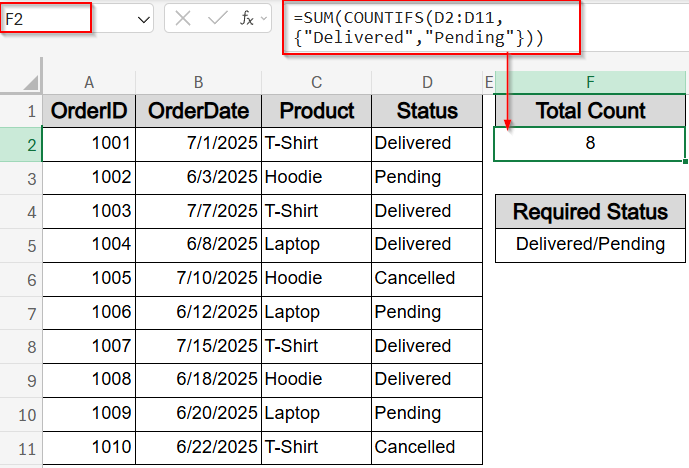
Excel will output the combined number of entries where the Status is either “Delivered” or “Pending”.
➤ Alternatively, enter the following in another blank cell to simulate OR logic between two separate COUNTIFS conditions:
=COUNTIFS(C2:C11,”T-Shirt”,D2:D11,”Delivered”) + COUNTIFS(C2:C11,”T-Shirt”,D2:D11,”Pending”)
This sums the count of “T-Shirt” items that have either of the two target statuses.
➤ Press Enter to get the result.
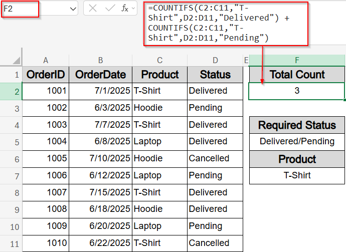
Now the formula returns how many “T-Shirt” orders were marked as either “Delivered” or “Pending”.
Add Logical Operators with COUNTIFS Function for Conditional Filtering
The COUNTIFS function supports a range of logical operators such as >, <, =, and <> which let you apply custom filtering rules across your data. This is especially useful when you need to exclude certain values or track entries that meet numeric thresholds or specific status flags.
In this method, we’ll use the <> (not equal to) operator to count how many orders have a status that is not “Pending”. This is helpful for quickly identifying how many orders are either completed or cancelled in our dataset.
Steps:
➤ Click on a blank cell such as F2.
➤ Type the formula:
=COUNTIFS(D2:D11,”<>Pending”)
This formula checks column D (Status) and counts how many rows are not marked as “Pending“.
➤ Press Enter to get the result.
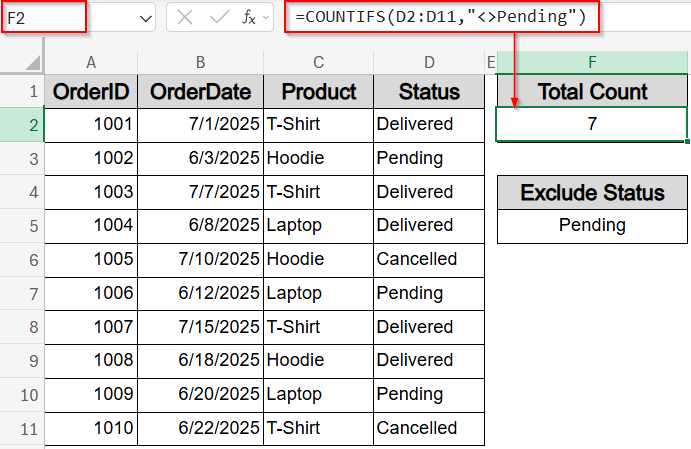
The output shows the total number of rows where the status is either “Delivered” or “Cancelled” excluding anything marked as “Pending“.
Insert COUNTIFS Function Inside an Excel Table with Structured References
Excel Tables allow you to create dynamic ranges that automatically expand as you add more data. When you convert your dataset into a Table, you can use structured references in formulas like COUNTIFS, making them easier to read and maintain. Structured references refer to column headers by name rather than using traditional cell ranges like A2:A11.
In this method, we’ll count how many orders in the table have the Product listed as “T-Shirt” and a Status of “Delivered.” The formula will update automatically as new rows are added, which makes this ideal for live reports and dashboards.
Steps:
➤ First, select your dataset range A1:D11.
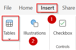
➤ Go to the Insert tab and click Table to convert the range into an Excel Table.
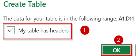
➤ Make sure “My table has headers” is checked and click OK.
➤ Excel will assign a default name like Table1. You can rename it from the Table Design tab if needed.
➤ In a blank cell like F2, enter this formula:
=COUNTIFS(Table1[Product], “T-Shirt”, Table1[Status], “Delivered”)
This formula uses the column names directly from the table to count rows where Product is “T-Shirt” and Status is “Delivered”.
➤ Press Enter to get the result.
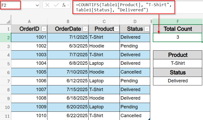
Now this dynamically counts matching rows and will automatically reflect any new data added to the table below row 11.
Frequently Asked Questions
What is the main advantage of using named ranges with COUNTIFS?
Named ranges make your formulas easier to read, maintain, and update. Instead of cell references, you use meaningful names, which reduces errors and improves clarity in complex spreadsheets.
Can COUNTIFS handle multiple OR conditions directly?
COUNTIFS function does not support OR logic natively. However, you can simulate OR conditions by summing multiple COUNTIFS formulas or by using array constants within the function.
How does COUNTIFS work with wildcards?
Wildcards like * and ? let you count partial text matches. For example, *apple* counts any cell containing “apple” anywhere. This helps when exact matches aren’t available or data entries vary.
How can I count dates within a specific month using COUNTIFS?
Combine COUNTIFS with DATE and EOMONTH functions to set dynamic start and end dates. This filters entries falling within the entire month without manually entering each date.
Why use structured references in Excel Tables with COUNTIFS?
Structured references automatically adjust as your table grows or shrinks, keeping formulas accurate without manual edits. They also improve readability by using column names instead of cell ranges.
Wrapping Up
In this tutorial, we explored advanced ways to use the COUNTIFS function in Excel for powerful data analysis. From dynamic date filtering and named ranges to wildcards, logical operators, OR logic, and structured table references, these techniques will help you handle complex datasets more efficiently and accurately. Feel free to download the practice file and share your feedback.