
In Excel, we often need to work with data that is larger or has skewed trends. This makes it harder to analyze that large numeric range, let alone identify its trends. Transforming these numbers into log is exactly used in data analysis reports, business reports on normal distribution, stabilize variance, or highlight underlying data trends. Usually, the patterns hidden in normal numbers are exponential growth and financial returns. Applying a log transformation in this situation makes the data readable and meaningful.
o log transform data in Excel, follow the steps below –
➤ Open the dataset and decide which column you want to transform.
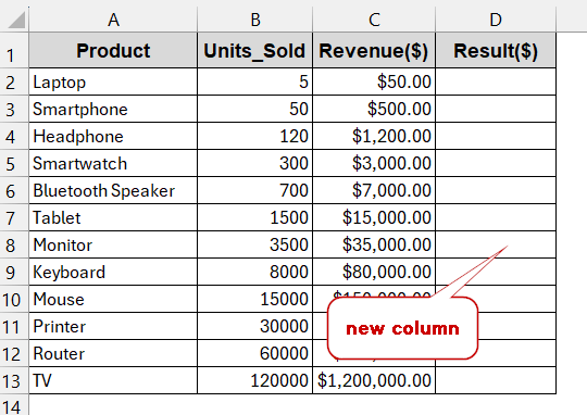
➤ Add a new column where you need to store the results.
➤ In the first column, write the formula of the log function : =Log(C2, 10),
where the C2 is the cell containing the large numeric range.
➤ Press Enter to get the value in the result cell.
➤ Drag the cells or use Fill Handle to use the formula for the rest of the cells.
In this article, we will explore ways in which you can get rid of large numeric values with log transformation. We will walk you through the ins and outs of the basic LOG functions with default base 10 and various custom bases. For extra scientific analysis, we will also look into natural log functions like LN (with base e). Apart from that, we have also advanced non-formula methods achieved by VBA Macros and Power Query. Don’t be overwhelmed; these are quite simple methods. Stay with us to see yourself.
Using The LOG Function For Log Base 10
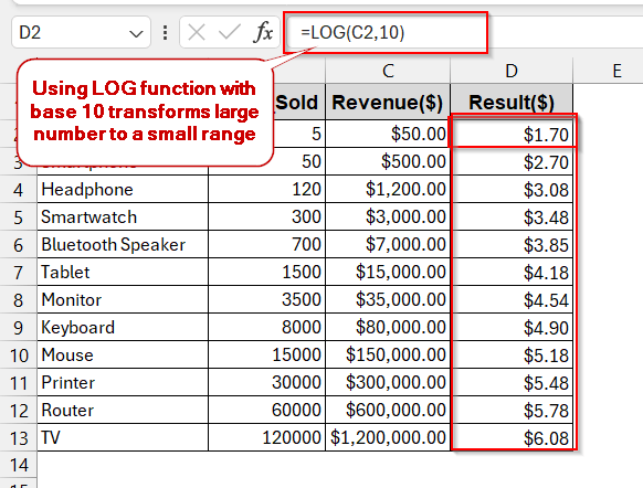
The most common way to transform the large numeric values is to use the LOG function with a base of 10. It is beginner-friendly, does not require complex steps, and can be done with some easy clicks. Using this, your data gets simpler and easier to interpret.
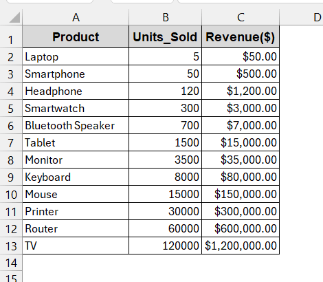
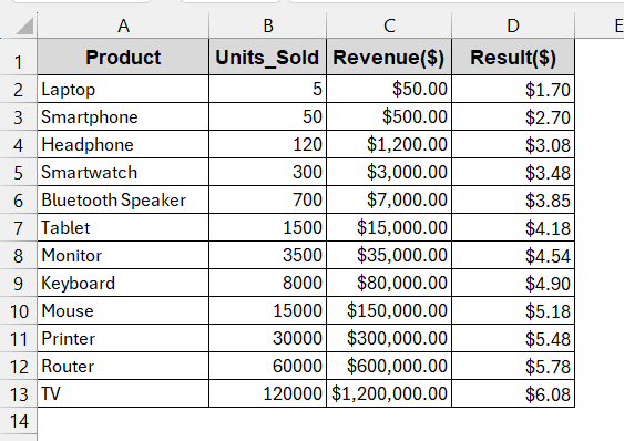
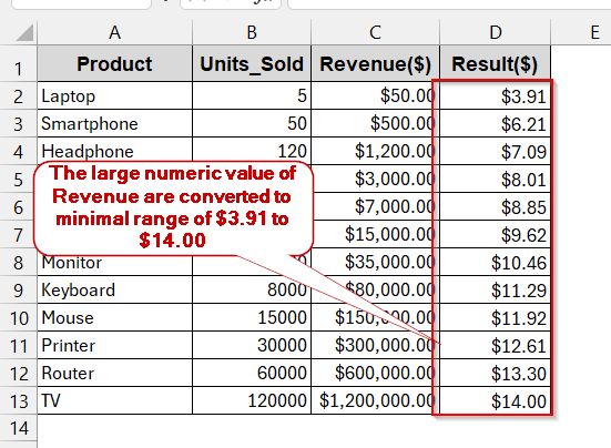
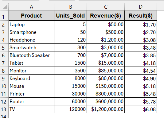
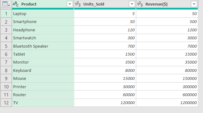
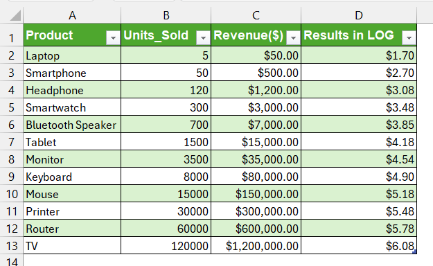
Here, we will use the dataset of product revenue with unit costs. The revenue values are between $50 to $1,200,000. This makes the range larger and quite complex to understand.
Thus, we will transform the Revenue into logarithmic numbers to determine their trends.
Steps:
➤ Open the datasets and find the column that needs to be transformed.
➤ Create a new column to enter the transformed values.
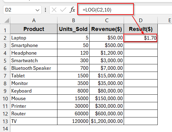
➤ Write the LOG function in the first cell of the column-
=LOG(C2, 10)
Here, the C2 cell is the first cell of the Revenue column that will be passed into the logarithmic values.
➤ Press Enter to get the results.
➤ Drag the cells to apply the same formula to all the other cells.
You can format the cell as you require later on.
Notes:
Excluding the base 10 parameter from the formula and writing only the column name also gives the same result. Excel LOG default functions transform a number to the logarithmic base 10.
Applying LOG with Different Bases
Not all the time, we want to transform our data to logarithmic base 10 values. Based on our needs, for example, in computing or information theory, you might need to convert the numeric value to custom bases. Luckily, that can also be done with this same LOG function.
In this method, we will be transforming the Revenue again, but this time with base 2.
➤ Open the dataset and create a result column to store the data.
➤ Locate which column has a large range of values.
➤ In the new column, write the formula of the LOG with the first cell reference of the required column –
= LOG(C2, 2)
Here, the C2 is the first cell of the column Revenue.
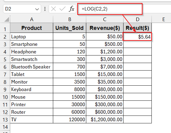
➤ Press Enter to get the result.
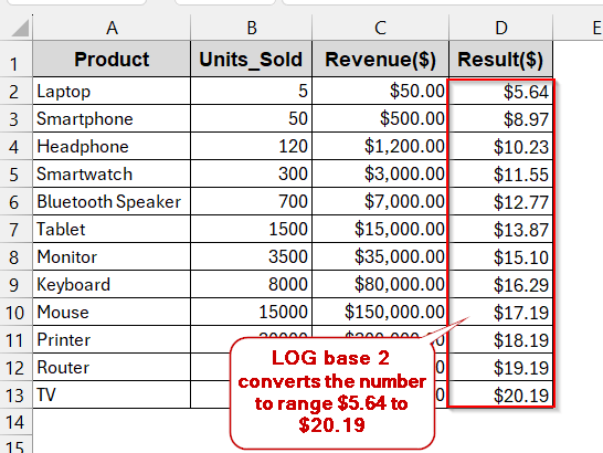
➤ Drag the cells to get the logarithmic range for the rest of the column.
Note:
The negative values will give #NUM! Error, as the logarithm base 2 gives undefined values for these ranges.
Working with the LN Function for Natural Log (Base e)
Instead of the LOG function, you can also use the natural log function of LN. Unlike base 10, it converts the number into a logarithmic base e. This model of the transformation is commonly used in scientific research and mathematical calculations to keep the data in the minimum range.
Steps:
➤ Open the datasheet and identify the column with the large numeric range.
➤ Create a new column to store the values.
➤ Use the LN function with the first cell of the column you need to transform –
=LN(C2)
Here, C2 is the first cell reference of the Revenue that needs to be transformed.
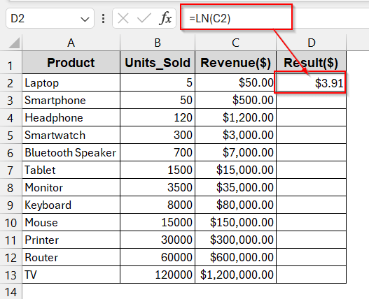
➤ Press Enter to get the result into the desired cell.
➤ Drag or use the Fill Handle to do the same for the rest of the cell in the column.
Notes:
The LN function only works with positive numbers. Zero or negative values will give a #NUM! Error.
Log Transformation with VBA Automation
When you need to work with large datasets, manually writing the LOG/LN function is repetitive and, of course, not productive. You might want to shift to an automated method, which will transform as many rows under the log functions as possible. In VBA Macros, you can write a short code snippet and get the entire column dealt in seconds.
Steps:
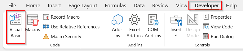
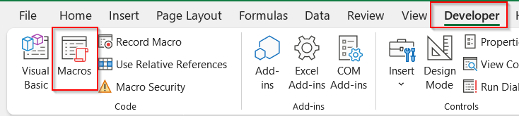
➤ Open the worksheet and go to the Developers tab -> Visual Basic.
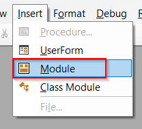
➤ In the launched VBA editor, click the Insert menu. Choose the Module option from there.
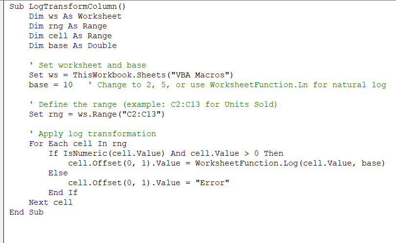
➤ In the blank space, write the following VBA code –
Sub LogTransformColumn()
    Dim ws As Worksheet
    Dim rng As Range
    Dim cell As Range
    Dim base As Double
    ' Set worksheet and base
    Set ws = ThisWorkbook.Sheets("VBA Macros")
    base = 10   ' Change to 2, 5, or use WorksheetFunction.Ln for natural log
    ' Define the range (example: C2:C13 for Units Sold)
    Set rng = ws.Range("C2:C13")
    ' Apply log transformation
    For Each cell In rng
        If IsNumeric(cell.Value) And cell.Value > 0 Then
            cell.Offset(0, 1).Value = WorksheetFunction.Log(cell.Value, base)
        Else
            cell.Offset(0, 1).Value = "Error"
        End If
    Next cell
End Sub
➤ Press Ctrl + S to save the VBA code and close the window.
➤ In Excel, click on any cell of the Result column, go to the Developers tab again, and now select Macros.
➤ In the Macro window, select the name of the VBA custom formula you created. In this example, our formula is logTransformColumn. Select it and click on Run.
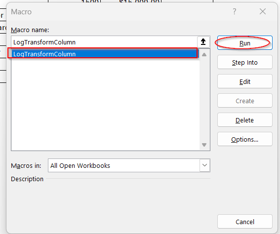
➤ The Macro will instantly produce log-transformed values in the Result column.
Notes:
➨ You can change the base of the LOG function by changing the base from line 7 –
base = 10 ‘ Change to 2, 5, or use WorksheetFunction.Ln for natural log
➨ Replace ‘VBA Macros with your sheet name to produce the correct values in line 6 –
Set ws = ThisWorkbook.Sheets(“VBA Macros”)
➨ Change the column range with your column range that needs to be transformed from line 9 –
Set rng = ws.Range(“C2:C13”)
Applying Log Transformation with Power Query
If you are not too much into formulas or complex VBA methods, Power Query can be the simplest and fastest way for you. With this, you can import the dataset into the Power Query tool, transform it into logarithmic numbers, and finally reload it.
Steps:
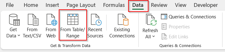
➤ Open the dataset and select the complete table.
➤ Go to the Data tab. Under the Get and Transform group, select From Table/Range.
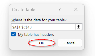
➤ In the dialog box, check the range properly. Check the box ‘My table has headers’.
➤ This makes a copy of the data into the Power Query Editor and enables users to edit in that virtual window.
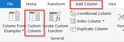
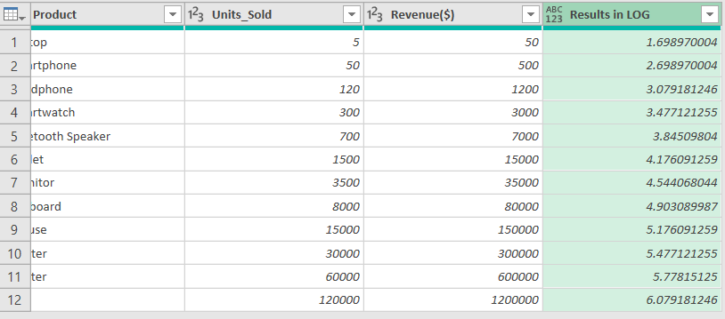
➤ Now, go to the Add Column tab -> Custom Column from the Power Query window.
➤ In the Custom Column window, give the new column a proper name. Write the formula in the formula box –
=Number.Log([#”Revenue($)”],10)
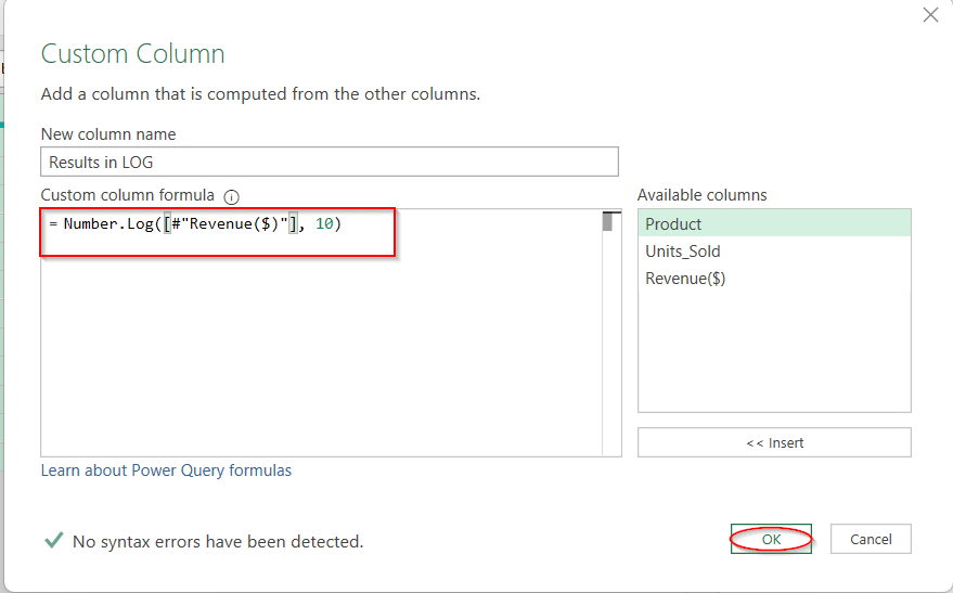
➤ Clicking OK will generate a new column with the log-transformed values of column Revenue into the Power Query.
➤When done, click on Close and Load on the Home tab of the editor.
➤ This will reload the table to a separate worksheet with the new column added.
The formatting is lost after the table is reloaded from Power Query. Reapply the necessary formatting of the columns,
Visualizing Log Transformed Data with Charts for Clearer Interpretation
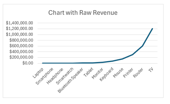
As you see, the large numeric ranges are often transformed through log transformation due to their clear data projection and interpretation. When making charts, these large values are often misleading, and growth trends often appear flat. For this reason, creating charts with the log values rather than the raw ones makes it much easier to see the underlying trends.
Here, we will be comparing two charts – one with raw Revenue and another with logarithmic values of Revenue. Both of them are put against the products to determine their trends. That means, the Products are in the x-axis and the Revenue on the y-axis.
Steps:
➤Select two columns, Product and Revenue (raw data).
➤ Go to the Insert tab. Under the Charts group, you can go for either a Line or Column Chart for a better view.
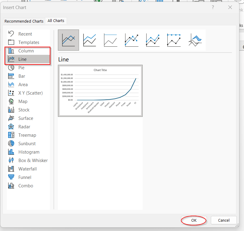
➤ Pressing OK will generate the chart with the raw data, which shows the value growing exponentially. Unfortunately, this does not give us enough information about the Revenue increase, especially for the preliminary stage.
➤ Now, make another new column by transforming the Revenue data to a log function. Use any of the five methods explained above.
➤ Then select the Product column and the log-transformed column. Go to the Insert tab and create another Line Chart for that.
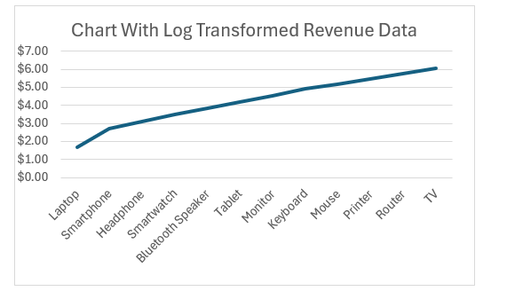
➤ When you put two charts side by side, you can see the latter one projects the trend much more clearly. It helps to see how the revenue is rising gradually, and at what rate the rise is occurring. This detailed view was lacking in the chart with the raw data.
Frequently Asked Questions (FAQs)
What is the difference between LOG and LN in Excel?
The LOG function transforms the values to any base you want. The default is 10, but you can customize your base per your needs. On the other hand, LN function only transforms the values in natural logarithm, that is, in base e (2.718). Therefore, LOG is used in easier and flexible calculations while LN is used in scientific ones.
Can Excel calculate log for negative numbers?
Excel can not calculate the log for negative numbers. The LOG function is only applicable for the positives; zero and negative values are mathematically undefined. As a result, Excel gives #NUM! Error for these values. If your data has negative values, filtering them out or adding an offset before applying log transformations is better.
How do I apply a log transformation to an entire column at once?
To apply the log transformation to the column at once, you can use either VBA or Power Query. They are minimal and faster, and fill the entire column without any Fill Handle options.
When should I use a log scale instead of a log transformation?
Log scales are usually used to visualize data using charts. With the numeric values having large ranges, you can use log scales to make the chart more understandable. Conversely, the log transformations are mainly used in calculations, modelling, and further analysis.
Why does Excel return a #NUM! Error in log functions?
The Excel can return #NUM! Error in the log functions only when the base or the value is invalid. Logs can not have any negative or zero numbers as their base or input values.
Concluding Words
Log transformation is more than just any mathematical chapter – it is a powerful way to make sense of your data that is skewed, scattered, or unreadable. Analyzing sales performance, modeling growth calculation, or even preparing scientific research data, log functions can make your sheets cleaner with more interpretable data. Using basic formulas like LOG and LN to advanced ones like VBA, Power Query, and dynamic charts, you can easily unlock new insights into the raw data.
Now, it’s your turn: open the sheets and try out our methods. Download our workbooks, follow each step, and see how your data transforms into better decisions and future trends.