
When working with large datasets, you may need to identify the smallest value based on specific conditions like product type, region, or category. While Excel doesn’t offer a direct function like MINIFS in older versions, you can still achieve this with combinations of functions like MIN, SMALL, IF, FILTER, and more.
In this article, we’ll learn how to find the lowest value in Excel based on single or multiple criteria. We’ll also cover both classic array-based methods and modern formulas like MINIFS and FILTER-based AND/OR logic for dynamic filtering.
Steps to find lowest in Excel with Criteria:
➤ Go to a blank cell like F3.
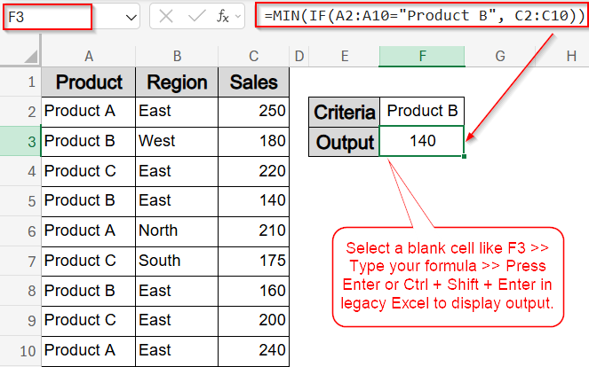
➤ Type this formula to find the lowest value for Product B:
=MIN(IF(A2:A10=”Product B”, C2:C10))
➤ Press Ctrl + Shift + Enter in legacy Excel, or just Enter in Excel 365.
Find Lowest Value with Single or Multiple Criteria Using MIN and IF Functions
When you’re using an older version of Excel (prior to Excel 2019), the MINIFS function won’t be available. In that case, use the MIN and IF functions together as an array formula. In this method, we’ll find the lowest value for both single and multiple criteria such as filtering by Product B only or including regional filters along with a specific product.
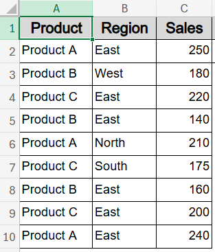
To demonstrate how to find the lowest value based on specific conditions, we’ll use a dataset that tracks product sales across different regions. The dataset includes columns for Product, Region, and Sales Amount, allowing us to apply various formulas based on one or more criteria.
Steps:
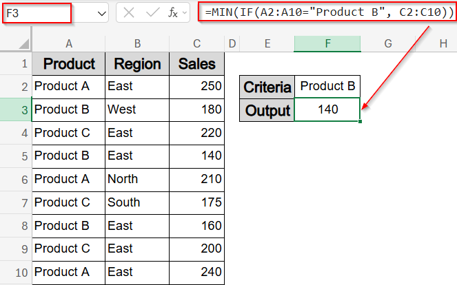
➤ Select a blank cell like F3 to find the lowest sales value for Product B only.
➤ In a blank cell, type formula:
=MIN(IF(A2:A10=”Product B”, C2:C10))
➤ Press Ctrl + Shift + Enter in legacy Excel, or just Enter in Excel 365.
➤ To include an additional condition, such as Product B in the East region, type this formula:
=MIN(IF((A2:A10=”Product B”)*(B2:B10=”East”), C2:C10))
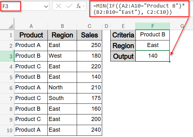
This formula finds the smallest value from the Sales column where both the Product and Region match the criteria.
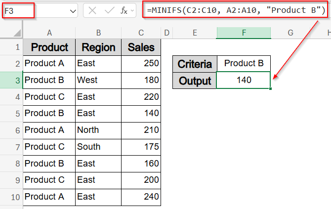
Use MINIFS Function for Simple Built-In Filtering
If you’re using Excel 2019 or newer, the MINIFS function is the easiest way to find a minimum value with conditions. It directly supports single and multiple criteria without needing array formulas. For example, to find the lowest sales value for “Product B” sold in the “East” region, this method will instantly return 140 based on our dataset.
Steps:
➤ Select a blank cell like F3 to find the lowest sales value for Product B only.
➤ In a blank cell, type formula:
=MINIFS(C2:C10, A2:A10, “Product B”)
➤ Press Enter to see output.
➤ If you want to find the lowest sales value for Product B in the East, enter this formula:
=MINIFS(C2:C10, A2:A10, “Product B”, B2:B10, “East”)
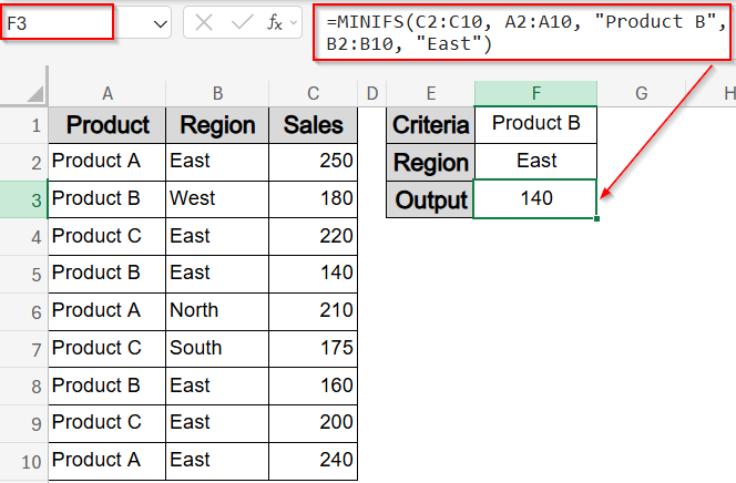
This returns the smallest number from the Sales column where the conditions for Product and Region are both met.
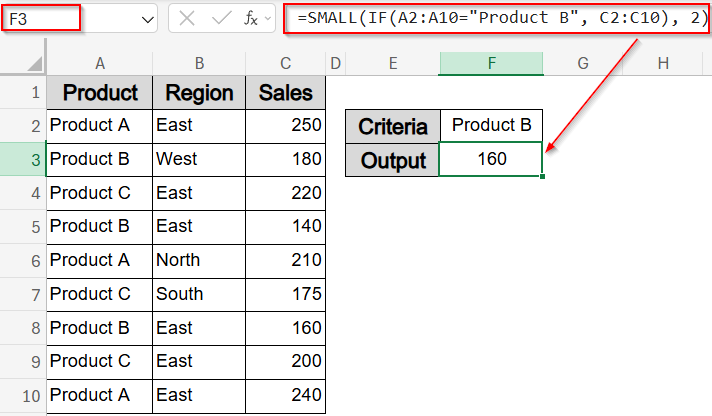
Find the Nth Lowest Value with Criteria Using SMALL and IF Functions
If you’re analyzing ranked data like identifying the second or third lowest sales for a specific product, the SMALL function combined with IF is an effective solution. This method filters the dataset based on your criteria and then returns the Nth lowest match. It’s especially useful when tracking top or bottom performers under certain conditions, such as the 2nd lowest sales for Product B, or the 2nd lowest sale where Product B was sold in the East region.
Steps:
➤ Select a blank cell like F3 to find the second lowest sales value for Product B only.
=SMALL(IF(A2:A10=”Product B”, C2:C10), 2)
➤ Use Ctrl + Shift + Enter in older Excel versions. Press only Enter in newer versions.
➤ To apply two conditions (Product B in East) for the second lowest and avoid errors neatly, use this formula:
=IFERROR(SMALL(IF((A2:A10=”Product B”)*(B2:B10=”East”), C2:C10), 2), “”)
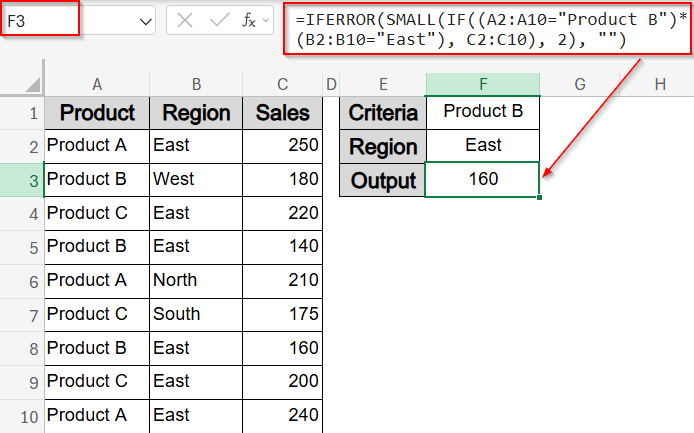
This helps when you’re doing rank-based filtering on criteria-matched values.
Filter-Based Minimum Using SMALL and FILTER Functions
For users working in Excel 365 or Excel 2021, combining the FILTER and SMALL functions provides a fast and elegant way to extract the minimum value based on one or more conditions. This method dynamically filters rows that meet your criteria like a specific Product and Region and returns the smallest value from the filtered results. Since it uses Excel’s dynamic array engine, there’s no need for Ctrl + Shift + Enter , and results update automatically when the data changes.
Steps:
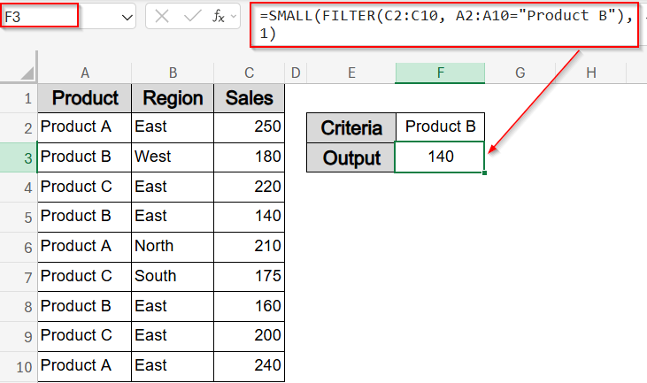
➤ Select a blank cell like F3 to find the smallest sales value for Product B only.
➤ In the blank cell, type formula:
=SMALL(FILTER(C2:C10, A2:A10=”Product B”), 1)
➤ Press Enter to see output.
➤ To filter by two conditions (Product B and East region), enter this formula:
=SMALL(FILTER(C2:C10, (A2:A10=”Product B”)*(B2:B10=”East”)), 1)
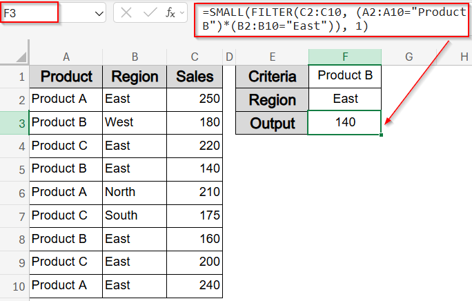
This modern approach avoids array-entering and returns a clean dynamic result.
Filter by AND / OR Conditions Using FILTER and SMALL Functions
This method lets you extract the lowest value based on multiple conditions either using AND logic (all conditions must be true) or OR logic (at least one condition must be true). It’s especially useful if you’re using Excel 365 or Excel 2021, where FILTER function is supported.
Let’s say you want to find the lowest sales value for Product B in the East region. You can do this with AND logic. Or, you might want the lowest sales for either Product A or Product B, this is where OR logic helps.
Steps:
➤ Select a blank cell like F3.
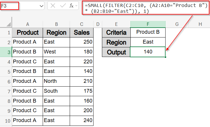
➤ To find the minimum sales where Product is “Product B” and Region is “East” using AND logic, type this formula:
=SMALL(FILTER(C2:C10, (A2:A10=”Product B”) * (B2:B10=”East”)), 1)
➤ Press Enter to see output.
➤ To find the minimum sales where Product is either “Product A” or “Product B” using OR logic, enter this formula:
=SMALL(FILTER(C2:C10, (A2:A10=”Product A”) + (A2:A10=”Product B”)), 1)
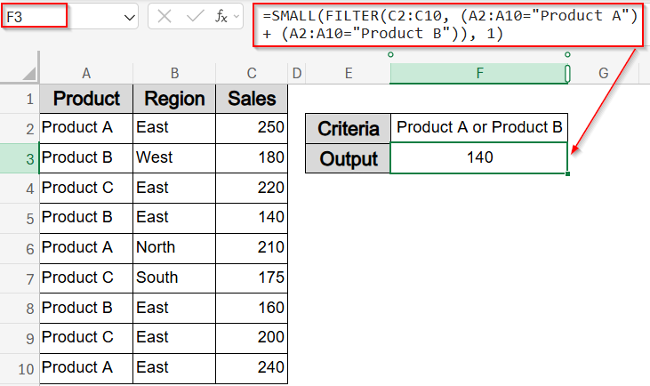
These formulas filter the Sales column by your criteria, then return the smallest matching value. Use an asterisk (*) between conditions for AND logic, and a plus (+) for OR logic. You can also replace hardcoded text with cell references to make them dynamic.
Frequently Asked Questions
Can I use MINIFS with multiple conditions?
Yes. The MINIFS function allows you to apply multiple conditions across different columns without needing array formulas. Each condition helps narrow the range until the lowest matching value is returned from the target column.
How do I get the 2nd or 3rd lowest value with criteria?
To retrieve the second, third, or any nth lowest value with conditions, use SMALL function combined with IF or FILTER function. Adjust the k value (e.g., 2 for second-lowest) to rank your filtered results properly.
What’s the difference between MIN and SMALL functions?
MIN function returns the absolute lowest value in a given range, while SMALL function returns the nth lowest value. SMALL function is more flexible when ranking results or retrieving a series of the lowest matching values.
How do I apply OR logic when filtering for lowest values?
Use a plus sign (+) between logical tests inside FILTER or IF function, such as (A2:A10=”A”) + (A2:A10=”B”). This includes any row that meets at least one of the specified conditions.
What happens if no matching value is found?
If your formula doesn’t find any values matching the criteria, it may return a #NUM! or #CALC! error. Wrap the formula with IFERROR function to replace errors with a message like “No Match Found” or leave it blank.
Wrapping Up
In this tutorial, we learned how to find the lowest value in Excel based on one or more criteria using functions like MIN, IF, SMALL, MINIFS, and the modern FILTER function. We covered both basic and advanced techniques, including how to retrieve the 2nd or Nth lowest value, and how to apply AND or OR logic for multiple conditions. Whether you’re working with older Excel versions or dynamic arrays in Excel 365, these methods help you extract the minimum values with precision and flexibility. Feel free to download the practice file and share your feedback.

