How to Use SUMIF Function to Sum Values Less Than 0 in Excel

When working with data in Excel, you’ll often find both positive and negative numbers. Positive values might represent income, sales, or gains, while negative values usually indicate losses, expenses, or deductions. If your goal is to quickly total only the negative numbers, Excel’s SUMIF function is the simplest way to do it.

This function allows you to apply conditions while adding values, making it especially handy for financial analysis, budget tracking, or inventory reports where you need to sum values less than 0.

Overview of the SUMIF Function in Excel

The SUMIF function in Excel is designed to sum cells within a range that meet a single, specific criterion. It sums values conditionally, like summing sales amounts for a particular product or totalling numbers greater than or less than a certain value.

Syntax:

SUMIF(range, criteria, [sum_range])

➤ range – The cells that Excel will check against the criteria.
➤ criteria – The condition determining which cells to include in the sum.
➤ [sum_range] (optional) – The cells that actually get summed if their corresponding range values meet the criteria. 

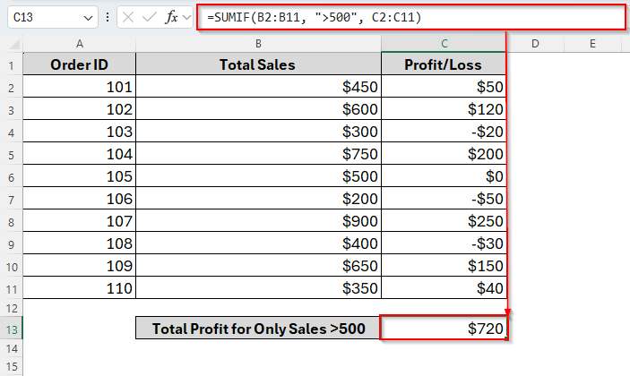
Example:

The easiest way to sum values less than 0 would be using the SUMIF generic formula in Excel. It’s very useful when we need to sum within a range using a single criterion. So, the generic formula for the SUMIF function is:

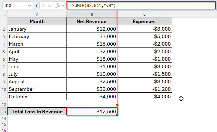
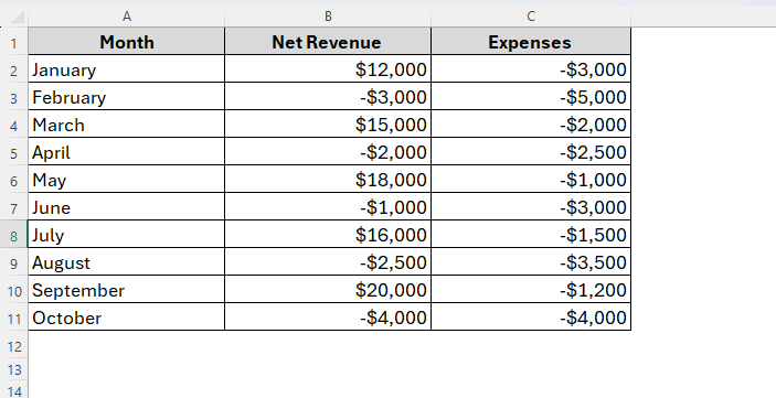
To understand it better, here we have a dataset showcasing a company’s monthly revenue and expenses based on each month. In this dataset, the Net Revenue refers to the monthly profit in positive numbers and loss in negative numbers. And the column Expenses includes only negative numbers indicating outflows.

So, let’s say we’ll sum Net Revenue only for loss, which means the negative numbers or values less than 0. And here, we’re going to apply the SUMIF generic formula by the following steps.

Steps:

➤ Select the cell B13.
➤ Now insert the following formula in the cell:

➤ Hit the Enter key and here’s the total revenue for months where there’s only loss.

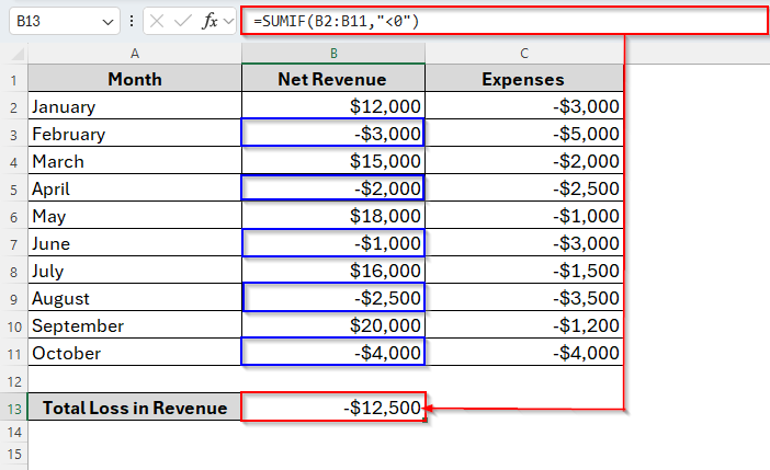
That means once we apply the formula, it only counts the negative numbers from column B. In this way, we can sum only negative numbers or values less than zero for any range from any dataset.

In the previous method, we just counted the total revenue for loss. But what if you need to sum the expenses in column C for any month where the net revenue in column B is less than 0? Well, the SUMIF function in Excel also allows us to sum negative numbers based on the condition of a different column.

Based on today’s dataset, for example, now we’ll sum total expenses when the net revenue is only on negative numbers. So, let’s see how it goes.

Steps:

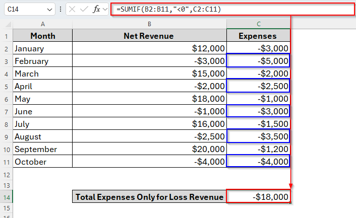
➤ To begin with, type the formula as follows in cell C14:

➤ Tap Enter. And we’ll get the total expenses only for loss revenue in column B as you can see in the image below.

In the previous two methods, we’ve used hardcoding conditions in the formula like <0. But you can also use a cell reference in the SUMIF formula instead of hardcoding the condition. Here we put the condition value in a separate cell, and then refer to that cell in your formula.

By doing so, if you want to change the condition later, like from >0 to >100, you don’t need to edit the formula again. You just have to change the value inside that cell, and Excel will automatically update the result.

Now, in this method, we’ll show how to sum values less than 0 using a reference cell.

Steps:

➤ Firstly, insert the criteria 0 in cell C13.
➤ Then, enter the following formula in cell C14:

➤ Press Enter and here we got the same result as the previous method. That means it counts the total expenses in Column C, when the Net Revenue is less than 0 from Column B.

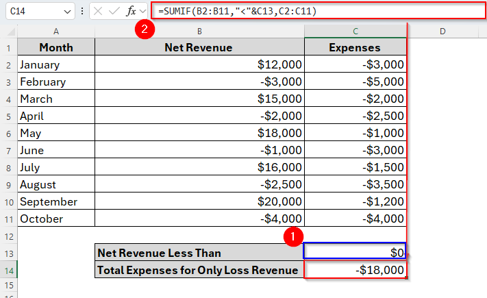
But instead of using the criteria <0 in the formula, we applied the cell reference C13.

As we already know, the SUMIF function in Excel allows us to use a single criterion. But sometimes we may also need to apply multiple criteria based on the dataset. In this case, we can use the SUMIFS function. With this function, we can apply more than one criterion in a formula.

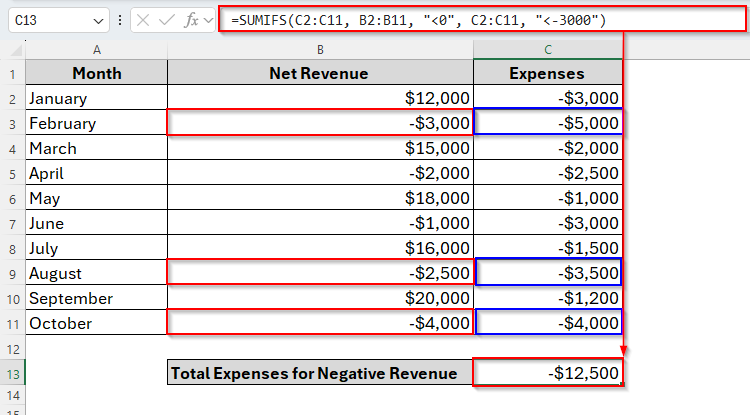
For instance, now we’ll sum expenses from column C for months with negative revenue (column B) and a total expense less than -$3,000 (column C). Here, we’ve two different criteria. One is less than 0 and another is less than -$3000. So, let’s see how we can insert the SUMIFS function while combining these two criteria.

Steps:

➤ In cell C13, insert the formula as follows:

➤ Tap Enter. And here’s the total expenses for negative revenue under $-3000.

Frequently Asked Questions

Why is my SUMIF formula returning 0 even though I have negative numbers?

The key reason for this problem is that the numbers may be stored as text. So, convert them into numbers. Moreover, there might be spaces or hidden characters in your cells. Use TRIM() or clean the data.

Can I use SUMIF for multiple conditions like less than 0 and greater than -100?

SUMIF only supports one condition. To apply multiple conditions, you should use SUMIFS instead.

What does the SUMIF function do in Excel?

The SUMIF function adds up values in a range based on a condition you specify. For example, you can sum only the negative numbers (less than 0), only positive numbers, or only values that meet certain criteria.

Concluding Words

This is how the SUMIF function makes it really easy to handle negative numbers in Excel. If you want to quickly find out the total of all losses, expenses, or any other values that are less than 0, this function is the perfect solution.

You don’t need to filter or sort your data manually, just set the condition <0 and Excel does the rest for you. Once you get comfortable with this function, you’ll save a lot of time and get clearer insights from your data.