While doing data analysis in a pivot table, arguably the most useful menu in Excel can be accessed from the PivotTable Analyze tab. This tab gives access to most of the tools you need to customize the pivot table data and complete your report. However, the tab might not show up when you need it the most, and having to deal with that can be frustrating.
There are some reasons why the PivotTable Analyze tab might not show up in Excel. In this article, we will learn the reasons for that and how to restore the PivotTable Analyze tab in your Excel sheet.
➤ Go to the worksheet where the pivot table is located.
➤ Select a cell of the pivot table.
Finding the PivotTable Analyze tab might not be as easy for your dataset. In this article, we will go through all of the solutions you can apply to find the PivotTable Analyze tab. Download the workbook we used in this article to practice the methods yourself. Let’s begin.
Activating the PivotTable by Selection
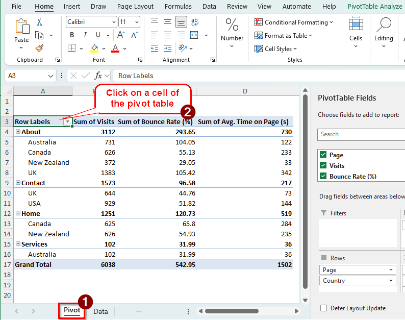
For demonstrating the issue, what pivot table we use does not matter; however, for the record, we have a pivot table with website traffic data. There are the page names, visits, bounce rates, average time people spent on pages, and the countries they visited from. We are in the new worksheet where we created the pivot table, but the PivotTable Analyze tab is not visible. Here is how to get it back:
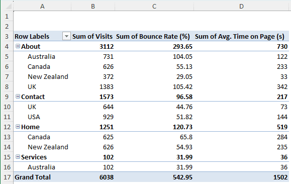
➤ The pivot table consists of A3:D17 cells. The sheet might be considered as a separate sheet for the pivot table; Excel does not show the pivot table-related functions until you select the pivot table.
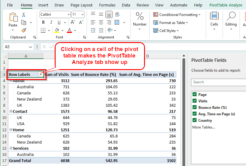
➤ Click on any cell inside the pivot table, i.e, the A3:D17 range.
➤ The PivotTable Analyze tab will show up now.
Resetting the Excel Ribbon
The PivotTable Analyze tab exists in the ribbon of Microsoft Excel, but it might go missing for some custom settings. A way of getting it back would be resetting the ribbon. Here is how to do it:
➤ Go to File > Options.
➤ In the new window called Excel Options, go to Customize Ribbon
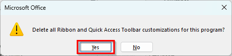
➤ Click on Reset all Customizations from the dropdown of Reset in the Customizations section.
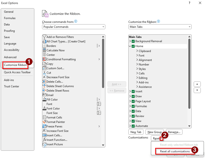
➤ Click Yes in the confirmation dialog, and OK in the previous window. This will reset the settings in the Excel ribbon, and the PivotTable Analyze tab will show up again when you select a cell in the pivot table.
Adding PivotTable Analyze Tab to the Ribbon
If resetting does not work, you can add the PivotTable Analyze tab manually to the ribbon. Here is how you can do that:
➤ Head to File > Options.
➤ In the new window, go to the Customize Ribbon section.
➤ Select Tool Tabs from the “Customize the Ribbon” dropdown menu.
➤ Check the box that says PivotTable Analyze and press OK.
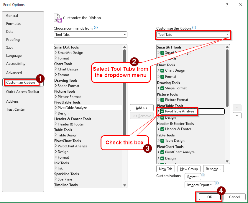
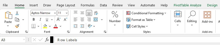
➤ Now the PivotTable Analyze tab will be available.
Making the Ribbon Visible
The PivotTable Analyze tab belongs in the ribbon. If the ribbon is not visible, the tab won’t be visible as well. Follow the instructions below to show the ribbon.
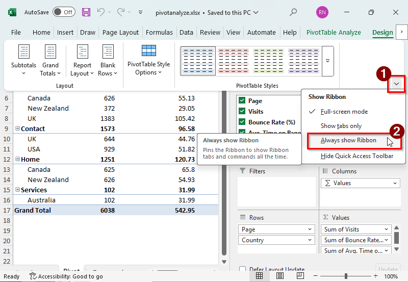
➤ Assuming Excel is in full-screen mode, click on the three dots in the top-right of the Excel window. This will show the ribbon temporarily.
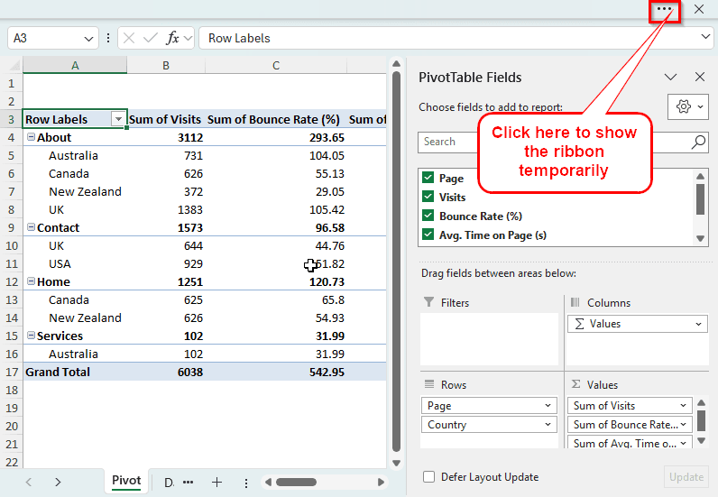
➤ Now click on the small arrow right under the ribbon to show the “Show Ribbon” pop-up.
➤ Select Always show Ribbon to make sure that the ribbon is always shown, and you can use the PivotTable Analyze tab.
Repairing Microsoft Office 365
If none of those solutions worked, we have no choice but to repair Microsoft 365. Excel will get repaired in the process, and everything will work fine.
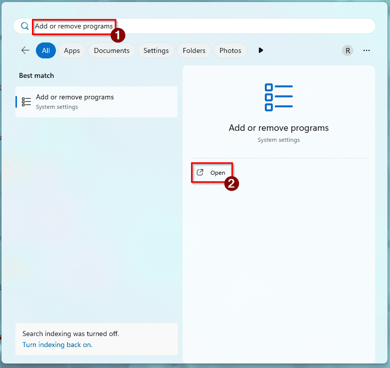
➤ Go to the start menu of Windows and search for “Add or remove programs”.
➤ Click Open.
➤ Search for Microsoft 365 in the Installed apps window.
➤ Click on the three dots to the right of the Microsoft 365 app and select Modify.
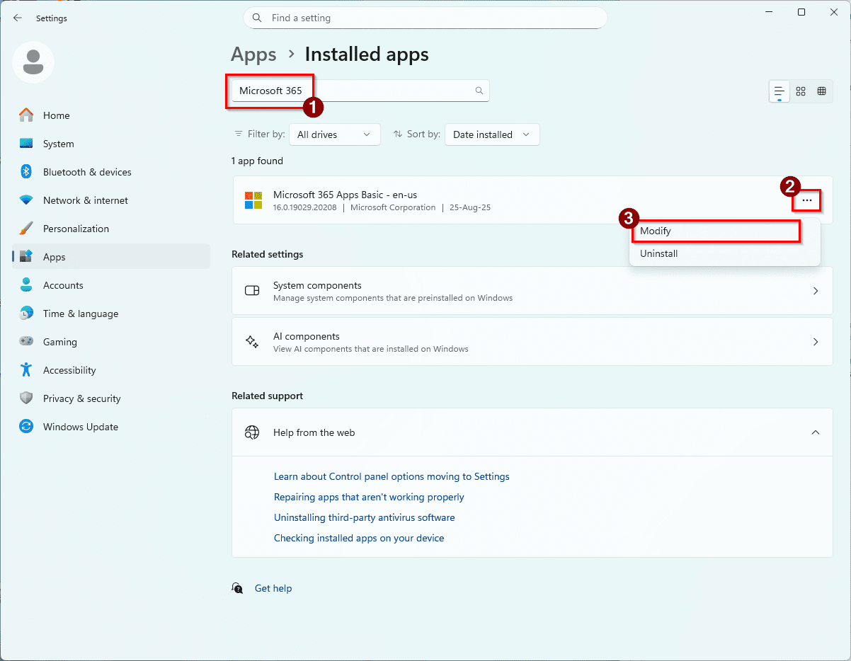
➤ Click Yes on the administrative prompt.
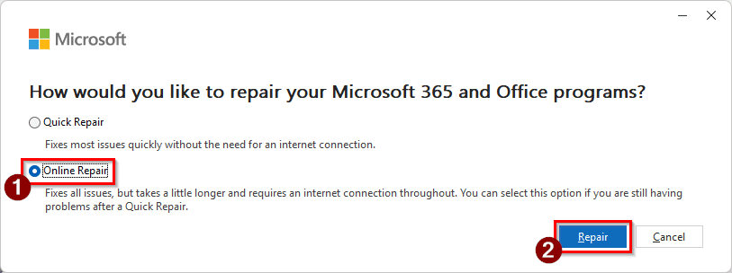
➤ Select Online Repair and hit Repair. Make sure you have an active internet connection. Microsoft 365 and Excel will be repaired, and every ribbon tab will work.
Frequently Asked Questions
Where is the PivotTable analysis button?
There is no button called “PivotTable Analysis”. However, there is a button called PivotTable Analyze, and it is located in the ribbon at the top of Microsoft Excel.
How to get PivotTable tools back?
Clicking on the pivot table should show the pivot table fields. If it does not, right-click on a cell of the pivot table and hit “Show Field List”. That should get you the tools for the pivot table back to your worksheet.
How to restore the Excel ribbon?
There are a few ways to do this. You can press Ctrl + F1 to restore the Excel ribbon. If the tabs are showing, you can double-click on any tab to restore the ribbon. In case it’s empty and Excel is in full screen, find the three dots in the top right corner of the window. Clicking it will give you options to restore the ribbon in Excel.
How to add pivot chart analysis in Excel?
Go to your table and select a cell, any cell at all. Then, head to the Insert tab of the ribbon. From there, select PivotChart. Select which chart you want to add, and press OK to confirm. A pivoted chart will be added to the worksheet.
Why is the table Design tab not showing in Excel?
A possible reason can be that the worksheet you are working with is protected. It can have protection from other people who made the file, or it’s protected because it was downloaded from the internet. If it’s the first case, you might need a password to unlock it. If it’s the second, you can just click Allow editing to fix it.
Wrapping Up
In this article, we have learned four methods to fix the pivot table analyze tab missing issue in Excel. If you still cannot find the PivotTable Analyze tab, leave a comment below, and we will look into it. For more Excel tutorials, visit our site anytime. We publish useful Excel guides regularly.