How to Do Ranking in Excel Pivot Table (4 Useful Ways)

Pivot tables are good for a lot of stuff in Excel. By pivoting a table, you can modify your data in various ways without changing the source table. In this article, we will learn how to rank in a pivot table. There are a lot of ways to do this in Excel, and in this article, we will show you step-by-step guides to do them for your convenience. After reading the article, you will be able to rank in a pivot table using the way you want.

Key Takeaways

➤ Right-click on the value field that you want to rank with.
➤ Go to Show Values As > Rank Largest to Smallest / Rank Smallest to Largest
➤ Select the base field for which you are going to rank.
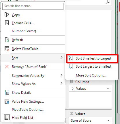
➤ Right-click the value field again, and go to Sort > Sort Largest to Smallest / Sort Smallest to Largest

Ranking is easy to perform in a pivot table, and there are numerous ways to do it. In this article, we will go through all of them so that you can learn the concept clearly.

Download Practice Workbook

Introducing the Dataset & Pivot Table

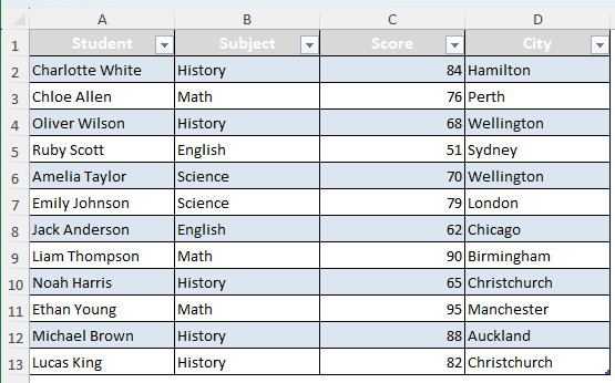
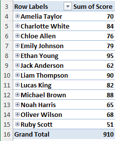
To demonstrate how to rank in a pivot table, we have a data table and a pivot table that we will use to apply the ranking methods. In our table, we have the scores of some students, the subjects they scored in, and the cities they live in. We want to rank the students based on their scores. Here are the methods to do that:

Data Table:

Pivot Table:

Sorting in Value Field Settings to Rank in a Pivot Table

This method is probably the easiest one to do, and it requires no formulas. Follow the steps below:

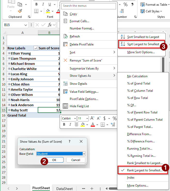
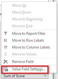
➤ The score is in the value field as Sum of Score. Click on it and select Value Field Settings.

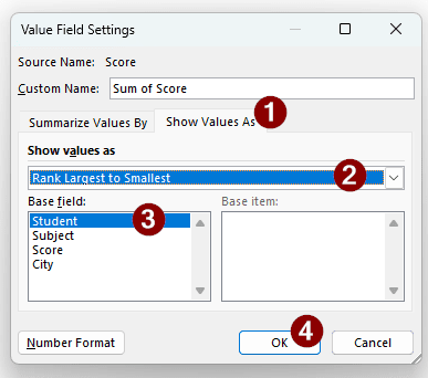
➤ In the Value Field Settings window, go to the Show Values As tab. In the dropdown, it would show No Calculation. Change it to Rank Largest to Smallest. Keep the Base field as Student. Press OK afterwards.

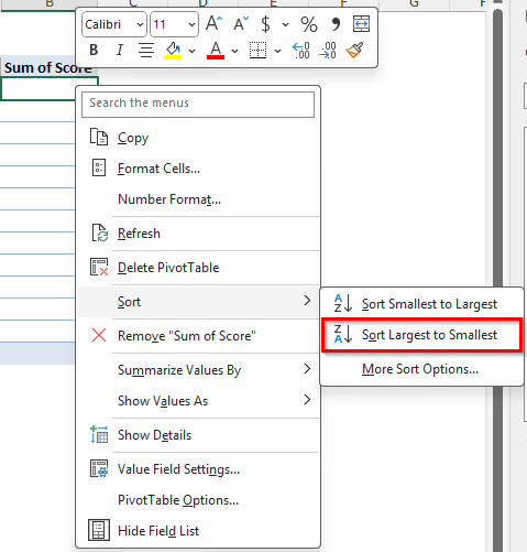
➤Right-click on any of the scores of the students, and select Sort > Sort Largest to Smallest.

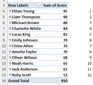
➤ If you have followed the steps correctly, the table will be formatted like the following:

Using a Calculated Field to Do the Ranking

In a pivot table, we can use a calculated field to modify the table instead of changing the source data. We don’t have to change the formatted data, and we can see the scores alongside the rank in this method. Follow the steps below to apply this method:

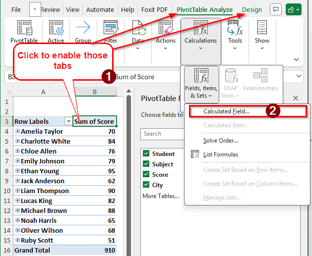
➤ Click on any cell of the pivot table so that the PivotTable Analyze and Design tabs get enabled.
➤ Go to Calculations > Fields, Items, & Sets > Calculated Field

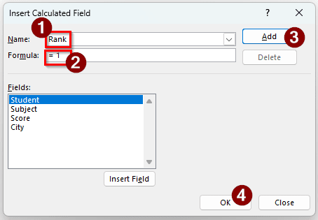
➤ In the Insert Calculated Field window, write Rank in the box called Name. In the Formula field, write = 1, and hit Add. Press OK to close the window.

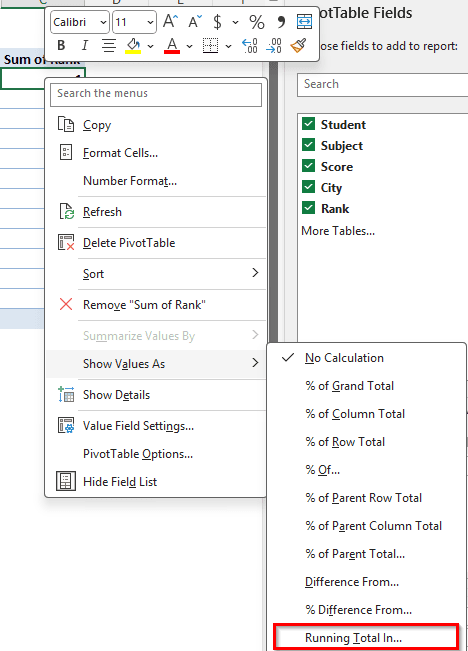
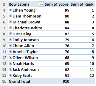
➤ Now, another column will be created called Sum of Rank, and all of its rows will contain 1.
➤ Right-click on any of the values in that column, and select Show Values As > Running Total In…

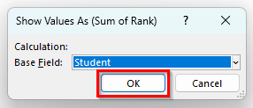
➤ A new window called Show Values As (Sum of Rank) will pop up. Keep the Base Field Student and hit OK.

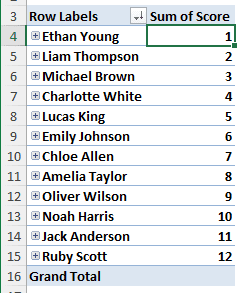
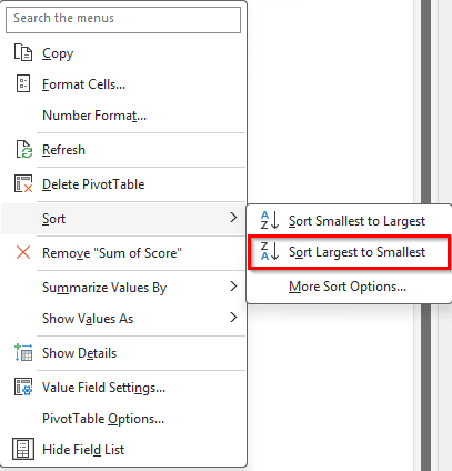
➤The rank is showing up in 1 to 12, but the scores aren’t actually ranked. To do that, right-click on a field of the Sum of Score, and select Sort > Sort Largest to Smallest.

➤ Now the scores should be ranked properly.

Inserting RANK Functions with the Pivot Table

Excel provides us with two ranking functions that we can use in our pivot table sheet. We don’t have to include them in our pivot table, but we can use them right beside our pivot table to do the ranking. Follow the steps below:

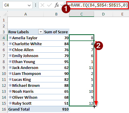
➤ Take a column right beside the pivot table. In this case, we have the A and B columns occupied by the pivot table, so we choose column C.
➤ Choose one of these formulas to write in the C4 cell:

=RANK.EQ(B4,$B$4:$B$15,0)

=RANK.AVG(B4,$B$4:$B$15,0)

=RANK(B4,$B$4:$B$15,0)

➤ Autofill till C15 cell.

Explanation

The RANK.EQ and RANK.AVG functions take three parameters. The first parameter is the cell that has to be ranked. In the C4 cell, we want to rank the B4 cell, and the cell will automatically change when we autofill.
The second parameter is the range it has to rank against. We use absolute references for the $B$4:$B$15 cells because we don’t want them to change when we autofill. The third parameter is the order for ranking, 0 means descending and 1 means ascending.
The difference between RANK.EQ and RANK.AVG is that RANK.EQ does not use average ranks for ties, so it does not contain floating-point rankings. In RANK.AVG, you can have a ranking of 4.5, but RANK.EQ will give you 4. The RANK function is deprecated and should not be used unless your Microsoft Excel version is older than 2010.

➤ Sort the scores from largest to smallest as you did before.

➤ Now the ranking will show up properly.

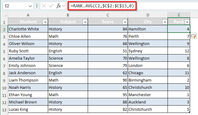
Changing the Source Table and Using RANK Function

Instead of modifying the pivot table, we can do the ranking in the source table by adding a column to it, and then pivoting the table.

➤ Add a column in the source table called RANK. We can just add the heading, and Excel will take care of everything else.
➤ Write either of the following formulas in the E2 cell. As it’s a table, we don’t have to autofill by ourselves; Excel will do that automatically upon pressing Enter.

=RANK.AVG(B4,$B$4:$B$15,0)

=RANK.EQ(B4,$B$4:$B$15,0)

=RANK(B4,$B$4:$B$15,0)

Explanation

Both of those functions take three parameters, as mentioned before. Here, the ranking is done for the C2 cell, which will dynamically change for other rows in the column. The second parameter is the range that will remain static. The third parameter asks the function to do descending ranking.

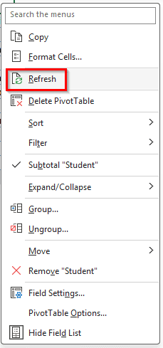
➤ Go to the pivot table, right-click, and hit Refresh so that the new column gets included in the table.

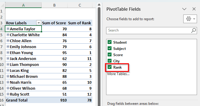
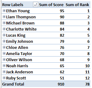
➤Select Rank from the PivotTable Fields panel on the right so that the Rank column shows up in the pivot table.

➤ Right-click on a cell from the Sum of Rank column, and select Sort > Sort Smallest to Largest.

➤ Now the pivot table values will be ranked.

Frequently Asked Questions

How to display a ranking in Excel?

There are two functions available in Excel to do that. The RANK.EQ function and the RANK.AVG function can be used to rank the numbers in your dataset. If you are using Excel 2007 or earlier, you can use the RANK function, but it’s deprecated in the newer versions of Excel. All of these functions take three parameters: The number to rank, the range to rank against, and the order or ranking.

How to show the top 5 items in a pivot table?

Click on the dropdown button of the Row Labels, and go to Value Filters > Top 10. In the new window, write 5 in the second field and click OK to show the top 5 items in your pivot table.

How to show the highest and lowest values in a PivotTable?

Click on a cell of the pivot table. Go to the Data tab of the top bar, and find the group called Sort & Filter. From there, select Sort Smallest to Largest or Sort Largest to Smallest. Now you will be easily able to notice the highest and lowest values in the pivot table.

Is rank the same as pivot?

No. Ranking is finding the position of a number in a list of numbers in ascending or descending order. A pivot table is a type of table used in Microsoft Excel to pivot the data from a source data range or a regular table.

What are the rank values in a table?

You can use the RANK, RANK.EQ, RANK.AVG functions to calculate the ranking in a table. The rankings will be based on the first parameter used in those functions.

Wrapping Up

We have learned ranking in a pivot table from this article. Using the methods mentioned in this article, you too can do this for your pivot tables. If you need, there is a box below to leave your questions. We will try our best to get back to you as soon as possible. Thank you for taking the time to read this article.

Post Views: 17