
In order to create a summary of all data, you might need to consolidate data from multiple worksheets into a single PivotTable. But this might be a little challenging and lead to errors if you manually copy and paste data into a single sheet. Excel offers several built-in tools that can summarize your data in a Pivot Table from multiple worksheets. In this article, we will walk you through three effective methods to consolidate data from multiple worksheets into a single PivotTable.
To consolidate multiple worksheets into one Pivot Table, here is one simple solution by using the PivotTable and PivotChart Wizard feature in Power Query.
➤ Press Alt + D + P shortcut to open PivotTable and PivotChart Wizard window.
➤ Choose Multiple consolidation ranges and PivotTable to create a PivotTable report.
➤ Select Create a single page field for me and click Next.
➤ Add all the data ranges from the worksheets and click Next.
➤ Choose New worksheet to create the PivotTable on a new sheet, combining multiple sheets.
Using PivotTable and PivotChart Wizard Feature
The PivotTable and PivotChart Wizard is a classic tool in Excel that can quickly consolidate data from multiple worksheets. Here, we will use the tool to add data from all sheets and create a single Pivot Table.
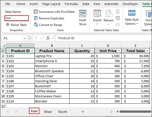
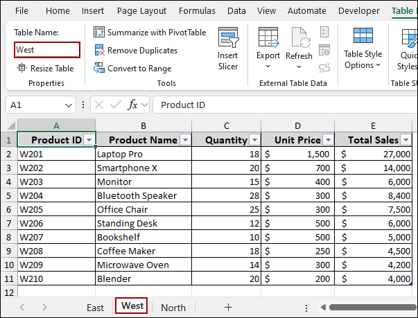
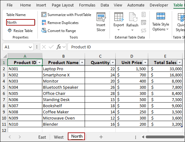
Let’s imagine we have three separate worksheets named East, West, and North, each with sales data that we want to combine. The data from all the worksheets is converted into a table and named according to the worksheets.
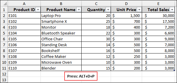
➤ Press Alt + D + P shortcut on your keyboard to launch the “PivotTable and PivotChart Wizard“.
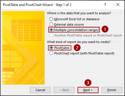
➤ Choose “Multiple consolidation ranges” to indicate that you want to combine data from different locations.
➤ Next, select “PivotTable” to create a PivotTable report.
➤ Click Next.
➤ Select “Create a single page field for me“.
➤ Click Next.

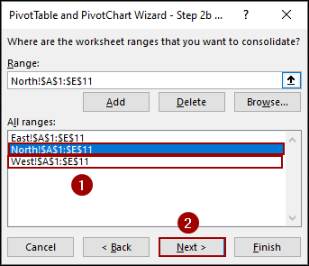
Now, you need to add the data ranges from each of your worksheets.
➤ Go to your first worksheet (e.g., East) and select the data range (e.g., A1:E11).
➤ Click Add.
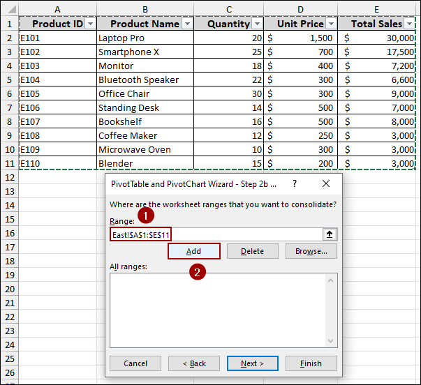
The range will appear in the “All ranges” box.
➤ Repeat this for each of your remaining worksheets (West and North).
➤ Then, click Next.
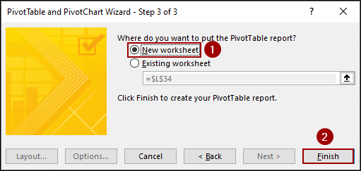
➤ Choose “New worksheet” to create the PivotTable on a new sheet.
➤ Click Finish.
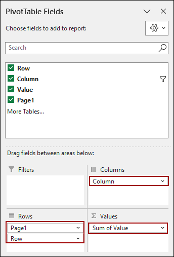
A new worksheet will open with a blank PivotTable and the “PivotTable Fields” pane. You will notice that the fields are named Row, Column, Value, and Page1.
➤ Drag the fields according to the image below.
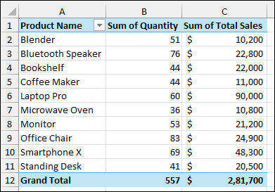
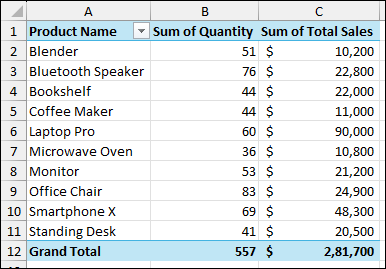
As a result, you will get the single Pivot Table consolidating data from the three worksheets.
Applying Append Queries Feature from Power Query
For a more dynamic solution, you can use the Append Queries feature from Power Query tool. This method works well when your data is not consistently formatted or when your data might change in the future.
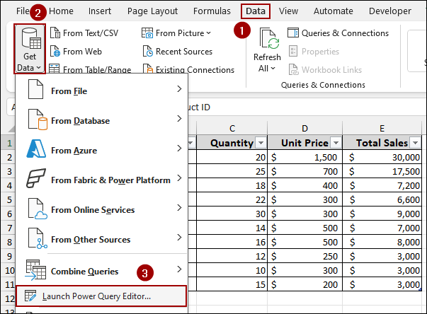
To begin, you need to open the Power Query Editor.
➤ Go to the Data tab on the ribbon.
➤ In the Get & Transform Data group, click Get Data.
➤ Click Launch Power Query Editor.
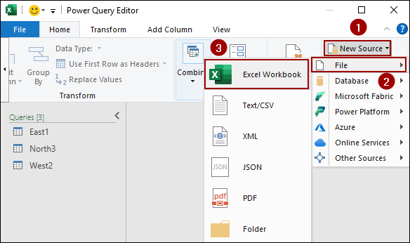
➤ From the New Source list, click File > Excel Workbook.
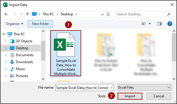
A file browser will appear.
➤ Locate and select your Excel file.
➤ Click Import.
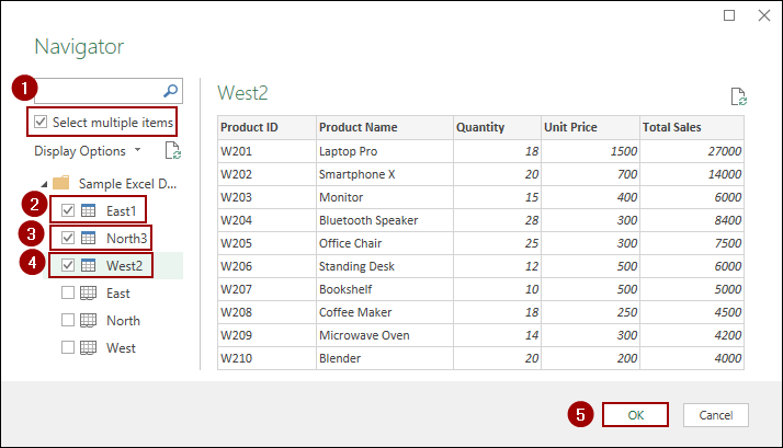
The “Navigator” window will now show all the sheets in your workbook.
➤ Checkmark the box for “Select multiple items“.
➤ Select the worksheets you want to consolidate (e.g., East, North, West).
➤ Click OK.
In the Power Query Editor, you will see a separate query for each of your selected worksheets. Now we need to append them.
➤ In the Combine group, click the dropdown menu and select Append Queries as New.
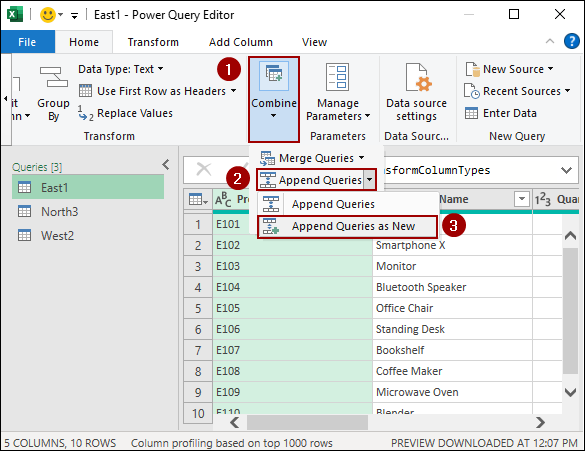
The “Append” dialog box will appear.
➤ Choose the “Three or more tables” option.
➤ Select the tables you want to append from the list (e.g., East1, North3, West2).
➤ Click Add to move them to the “Tables to append” list.
➤ Click OK.
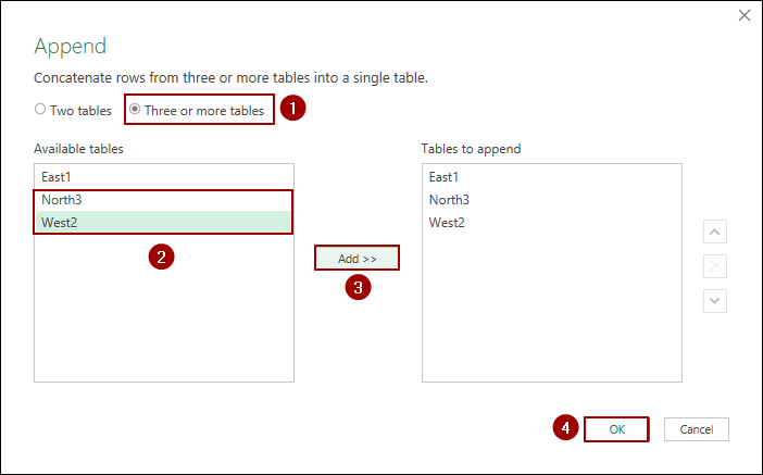
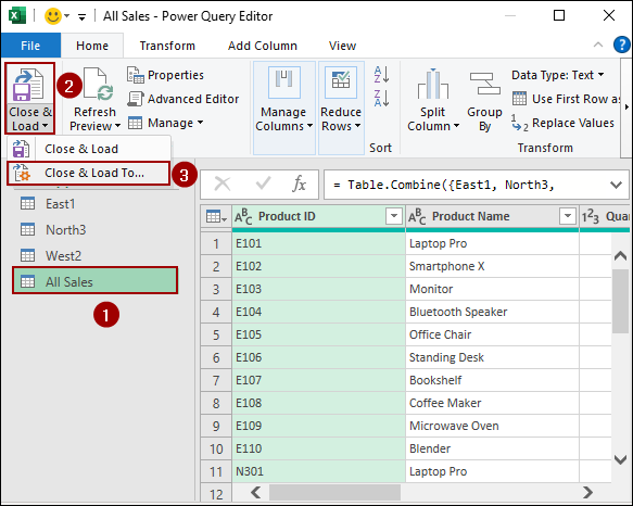
This will create a new query (e.g., Append1) containing all the data combined into a single table. Now that your data is consolidated, you can load it directly into a PivotTable.
➤ Change the Append1 name to All Sales.
➤ Click Close & Load To.
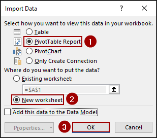
The “Import Data” dialog box will appear.
➤ Select “PivotTable Report“.
➤ Choose “New worksheet“.
➤ Click OK.
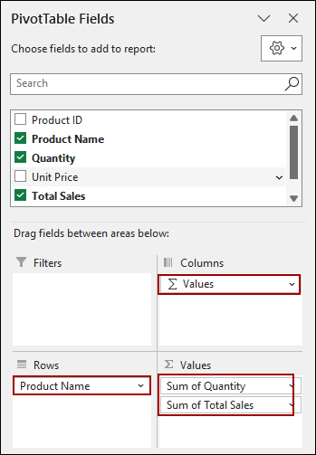
In the PivotTable Fields pane, you can now use the proper column headers from your consolidated data.
➤ Drag the Product Name field to the Rows area.
➤ Drag Quantity and Total Sales to the Values area.
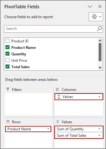
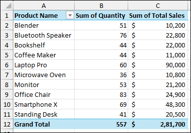
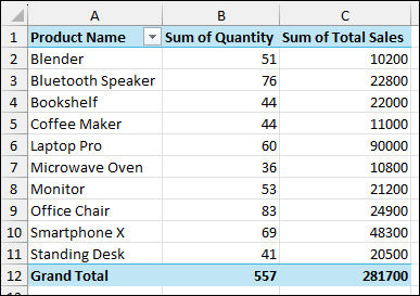
Finally, your PivotTable will now show the total quantity and total sales for each product, consolidated from all three worksheets.
Using Blank Query in Power Query Editor
You can also use a blank query to connect to the current workbook and consolidate all worksheets in one go. Here, we will create a new blank query, use a simple formula to connect all the worksheets and then create the Pivot Table.
➤ Go to the Data tab.
➤ In the Get & Transform Data group, click Get Data.
➤ Select From Other Sources > Blank Query.
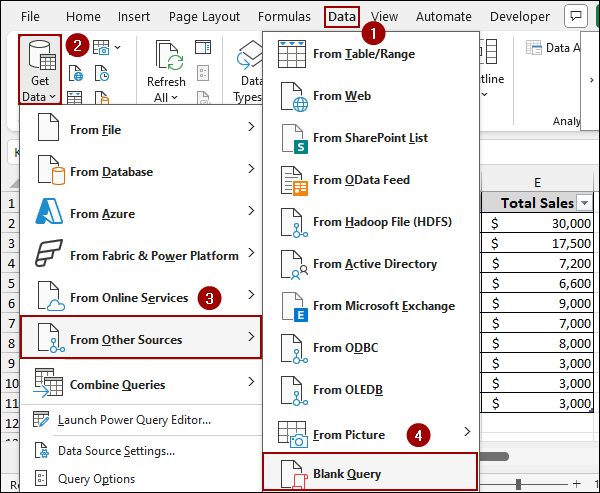
This will open the Power Query Editor with a blank query.
➤ Name the query as All Region Sales.
Now, we will use a simple formula to connect to all the data in the current workbook.
➤ In the formula bar, type the following formula.
=Excel.CurrentWorkbook()
➤ Press ENTER.
A table will appear, listing all the tables and named ranges in your workbook.
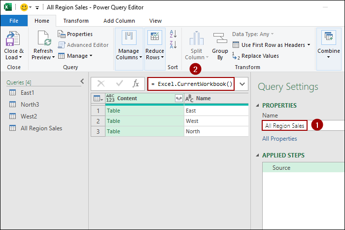
The table shows two columns: Content and Name. The Content column contains the actual data from each sheet. So, we will remove the Name column from the list.
➤ Right-click the Name column header.
➤ Select Remove Other Columns.
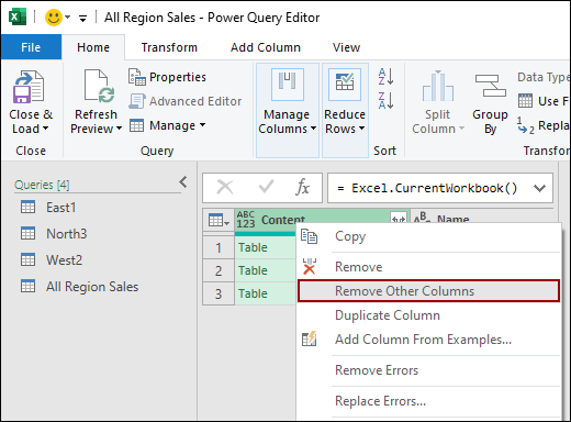
Now you are left with just the Content column.
➤ Click on the Expand icon (the two-headed arrow) on the Content column header.
➤ Uncheck the box “Use original column name as prefix“.
➤ Click OK.
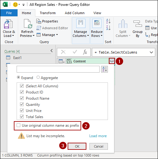
Power Query will expand the data, combining all your worksheets into a single, flat table. Now, you can load this consolidated data into a PivotTable.
➤ Go to the File tab.
➤ Click Close & Load To.
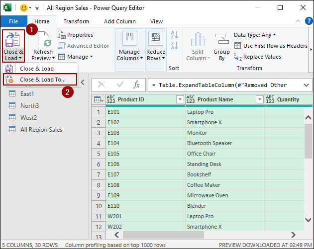
The “Import Data” dialog box will appear.
➤ Select “PivotTable Report“.
➤ Choose “New worksheet“.
➤ Click OK.
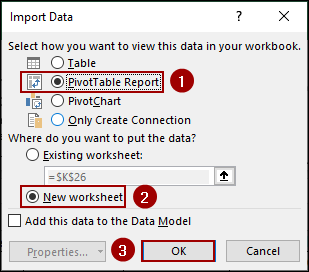
Thus, your new PivotTable will be created.
➤ In the PivotTable Fields pane, drag Product Name to the Rows area.
➤ Drag Quantity and Total Sales to the Values area.
The final PivotTable will display the consolidated sales data from all your worksheets.
Downloadable Resources
Get our practice workbook or necessary files that we have worked with to prepare this article.
Consolidate Multiple Worksheets into One Pivot Table.xlsx
Frequently Asked Questions
Can I update the Pivot Table if the source worksheets change?
Yes, if you use Power Query, you can refresh the Pivot Table to include updated or new data without recreating the Pivot Table.
What is the difference between using the consolidate tool and Power Query for Pivot Table consolidation?
The consolidate tool is simple but limited to basic calculations (sum, count, etc.) and doesn’t support dynamic updates well. Power Query is more flexible, dynamic, and recommended for larger or frequently updated datasets.
How do I handle duplicate records when consolidating multiple worksheets?
From the Power Query, you can use Remove Duplicates feature or add a unique key column to ensure only unique records are included in the final Pivot Table.
Concluding Words
Above, we have explored several ways to consolidate multiple worksheets into a single PivotTable. While the PivotTable and PivotChart Wizard is a quick and easy solution for simple tasks, Power Query offers a more dynamic approach that can handle complex data and future changes. If you have any queries, feel free to let us know in the comment section below.