Pivot tables are one of the oldest yet useful data analysis tools in Excel. The columns, rows, and values of a pivot table can be easily manipulated, which makes it a popular choice for data analysts. However, if the pivot table does not display all the required data for analysis, it can be frustrating. In this article, we will learn how to fix a pivot table that is not showing all data in Excel so that you don’t face any issues during your work.
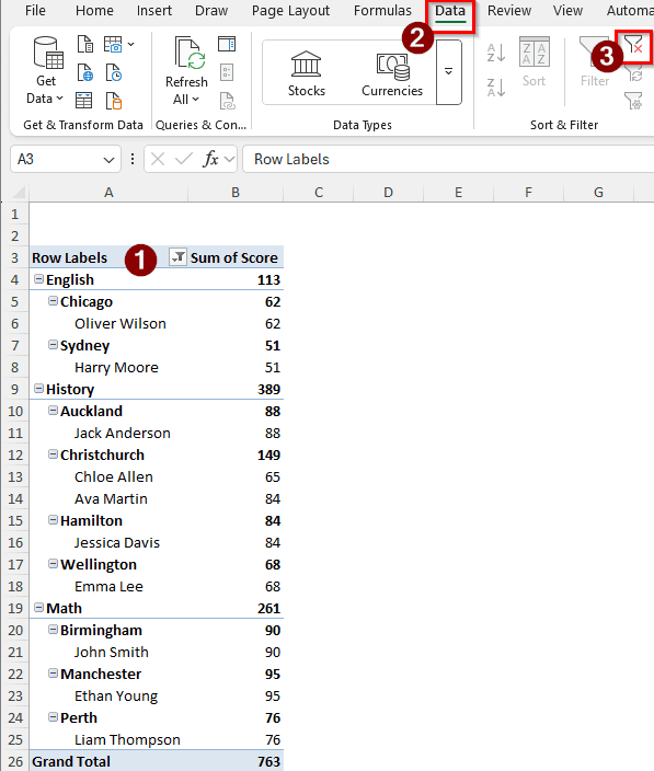
➤ Select any cell of the pivot table.
➤ Go to the Data tab in the Ribbon.
➤ In the Sort & Filter group, click on the Clear icon.
In most cases, that solution works pretty well. If it does not, you might want to read the other solutions we are going to provide in this article.
Clear the Filters
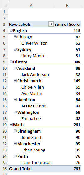
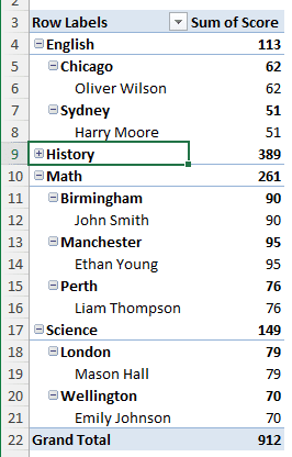
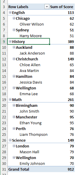
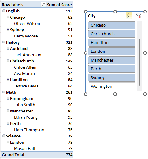
To demonstrate all the methods, we have a pivot table with some student grades. There are names of the students, their subjects, scores, and the cities they are from. In the pivot table, the subjects are listed at the top, yet we cannot see the students who chose science. The issue is, sometimes we have a filter on the pivot table that we don’t see in plain sight. The filter makes the table not show all the data. In order to fix that, we need to clear all the filters. Here’s how to do it:
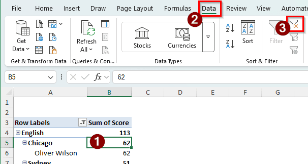
➤ First, select any cell from the pivot table so that we can manipulate the table.
➤ From the ribbon at the top, go to the Data tab.
➤ Locate the Clear button on the Sort & Filter group and click on it.
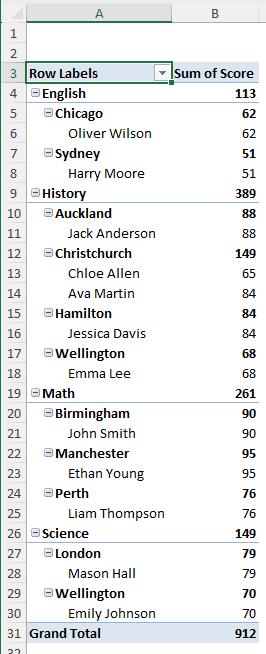
➤ Now the pivot table should show all the data.
Refresh the Table
After you add or modify the source data, the pivot table does not merge the changes to itself automatically. We have to refresh the table to make sure that the new data shows up. Follow the steps below to do it:
➤ There are three methods to refresh the pivot table. You can choose the one you are most comfortable with.
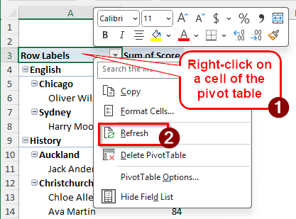
➤ The easiest method is to right-click on the table and choose Refresh.
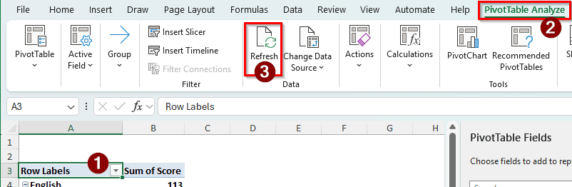
➤ You can also click on a cell to activate the pivot table and go to the PivotTable Analyze tab. Then, click on the Refresh icon to refresh.
➤ The third method is using keyboard shortcuts. Just click on a cell, and press Alt+F5 to refresh the pivot table. The pivot table will be updated, and everything you changed in the source table will show up.
Expand the Pivot Table
Sometimes, due to a misclick among other reasons, a pivot table can collapse and not show all the data. We need to expand it so that everything is shown properly.
➤ In the pivot table below, the history field is collapsed, so the students and the cities inside it are not visible.
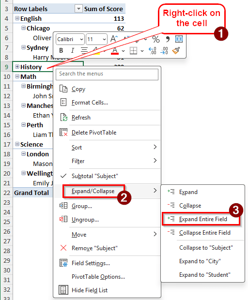
➤ We can right-click on the cell and select Expand/Collapse > Expand Entire Field.
➤ Now the field is expanded, and we can see the whole table.
Use the Proper Layout
Pivot tables are usually created in compact form. While this takes less space in the worksheet, it isn’t comfortable to view. Filters might go unnoticed when we have a compact form active. Changing the form to outline helps deal with this.
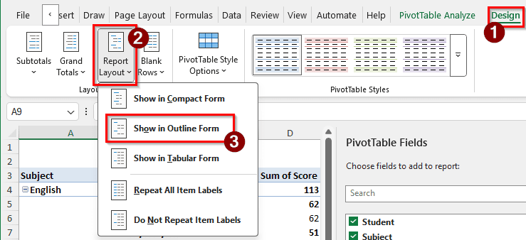
➤ When you have a cell of the pivot table selected, go to the Design tab.
➤ From the Report Layout button in the Layout group, select Show in Outline Form.
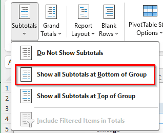
➤ While you are there, you might also want to select Show all Subtotals at Top of Group from the Subtotals section.

➤ To unhide the grand totals, select On for Rows and Columns from the Grand Totals section.
Enable Showing Items with No Data
If you have blank rows/columns, those won’t be shown in a pivot table by default. However, you can easily ask Excel to show them by following the steps below:
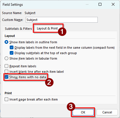
➤ In the PivotTable Fields section, click on your desired field, and go to Field Settings.
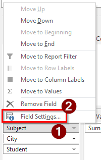
➤ In the Layout & Print tab, check the box that says Show items with no data, and hit OK.
Clear Slicer Filters
Slicers are not often noticeable in a pivot table. If we have filters enabled in a slicer, the pivot table will not show certain data in the worksheet. Here is how to clear slicer filters.
➤ Here, the data from Wellington is not shown because it is unchecked in the slicer.
➤ We can click on the small Clear button on the top right of the slicer to clear the filter. Then, the whole table will be visible.
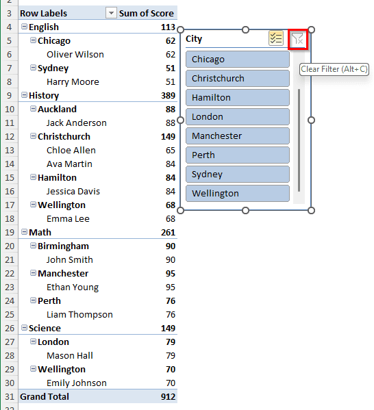
➤ You can also press Alt + C to clear the filter.
Frequently Asked Questions
Why is my PivotTable not reading all the data?
Check the data source and see if it’s corrupted or not. If the data source is okay, check whether all the data is included in the pivot table source. You can change the data source by going to the PivotTable Analyze tab in the ribbon and selecting Change data source.
Why is Excel not showing all fields in the PivotTable?
Right-click on the pivot table and select Show Field List to show the field list on the right. Then, from the PivotTable Fields panel, select all the fields that you need to see in the pivot table.
Why is my PivotTable only showing count?
The reason might be that the columns that you want to have calculated values in contain non-numeric data. Even if the rows have numerical data, they might not be formatted as such in the source table. Check the data source, then create a new pivot table to fix the issue.
Why is my PivotTable not showing totals?
To make the pivot table show totals, go to the Design tab of the ribbon and find the Layout group. On the left, you will find two buttons called Subtotals and Grand totals. Inside, there will be options to show totals in the pivot table.
How to expand PivotTable range?
To expand the range of the source data, you need to change the data source of the pivot table to the expanded range. Once you update the source, the pivot table will automatically expand to include that data. However, make sure that there isn’t anything other than blank cells in the sheet so that the pivot table can have enough space to expand.
Wrapping Up
In this article, we have learned six different ways to fix a pivot table that is not showing all data. We hope that these fixes will work for your dataset as well. Feel free to download the Excel file we used for the demonstration. We will see you in another article.