In Excel, a pivot table helps with formatting and customizing your data with a lot of options. If you made a pivot table, like the structure, but don’t want to keep the pivoting features of the table anymore, you are in the right place. In this article, we will learn how to remove pivot table but keep data.
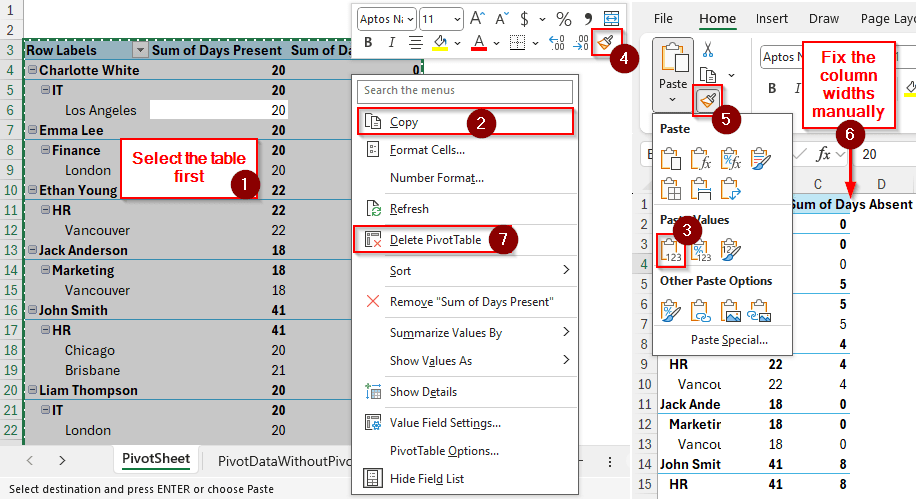
➤ Select the whole pivot table, right-click, and select Copy.
➤ Go to a new cell/sheet where you can paste this data.
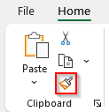
➤ From the Home tab, go to the Clipboard section and go to Paste > Values.
➤ Go to the pivot table back again, right-click, and select the Format Painter
➤ In the new table, select the Format Painter icon from the Clipboard section of the Home
➤ Set the column widths by yourself and delete the original pivot table.
That was a lot of steps, however, we have explained it in simple terms in this article. Moreover, we have another method that uses VBA and takes a lot less steps for a much better outcome. So, you might want to read the whole article to get a better understanding of the procedures.
Removing the Pivot Table but Keeping Data
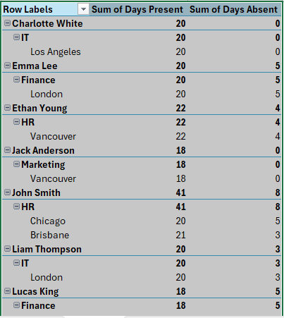
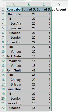
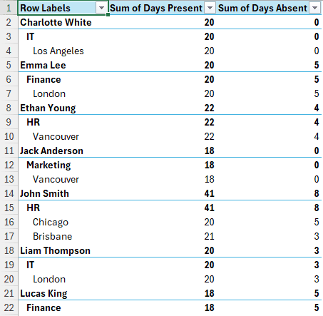
In this article, we have a pivot table of an attendance sheet for some employees. We have the sum of days absent and present, the employee names, the departments they work in, and the cities from which they are located. While the pivot table is created from a data table, we want to export this pivot table to a regular data range without keeping the pivot table. However, it is not possible to directly remove the pivot table while keeping the data, so we will copy the data to another location and delete the pivot table.
Step 1: Copy the Data
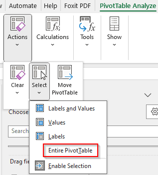
➤ Select any cell of the pivot table and go to PivotTable Design > Actions > Select > Entire PivotTable.
➤ Press Ctrl + C to copy the pivot table.
➤ Go to the new cell where you want to copy the data.
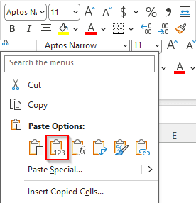
➤ Right-click on that cell and select the Paste Values icon.
Step 2: Copy the Format
➤ At this point, you should have the new data range selected. At the bottom of the Excel, it should still say “Select destination and press Enter or choose Paste”. If it does not, don’t worry, but you have to select the source pivot table again.

➤ Go back to the original pivot table, and select the Format Painter button from the Clipboard section of the Home tab.
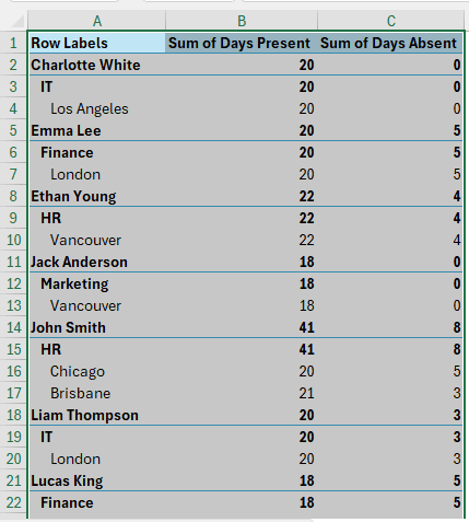
➤ Go to the new data range and click on the first cell of the data (A1 in this case). Now your table should look like this.
Step 3: Finishing Up
➤ Unfortunately, there is no way to copy the column width without keeping the pivoting features of the table. You will have to do that manually.
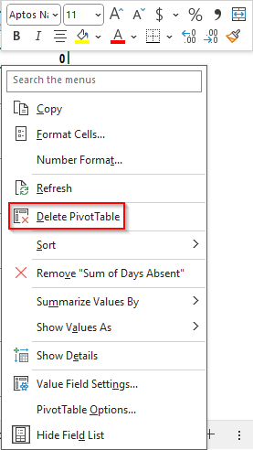
➤ Go to the original pivot table, right-click on any cell, and choose Delete PivotTable to remove the table.
➤ Select the new data range, and press Ctrl + T to create a regular table.
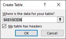
➤ Upon pressing OK, the colors and the style of the new table might change.
➤ To fix that, select any cell of the table and go to the Table Design tab.
➤ From the Table Styles/Quick Styles dropdown, select Clear.
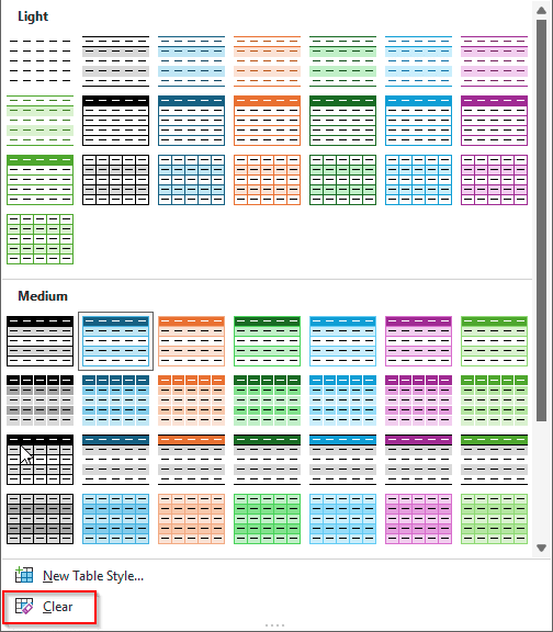
➤ Now the table should look and feel exactly like a regular table with data, but without the pivoting features.
Using VBA to Remove Pivot Table While Keeping Data
The manual procedure takes a lot of steps. However, using VBA code, we can cut down the steps and accomplish all the tasks in one go. Let’s see how to do that:
➤ Press Alt + F11 (Alt+Fn+F11 for some keyboards) when you are on the spreadsheet with the pivot table.
➤ Go to Insert > Module and write this code down:
Sub CopyPivotTableDataAndFormatToAnotherSheet()
Dim pt As PivotTable
Dim sourceWs As Worksheet
Dim targetWs As Worksheet
Dim rng As Range
Dim targetCell As Range
Dim i As Integer
Set sourceWs = ThisWorkbook.Sheets("PivotSheet")
Set targetWs = ThisWorkbook.Sheets("PivotDataWithoutPivotVBA")
If sourceWs.PivotTables.Count = 0 Then
Exit Sub
End If
Set pt = sourceWs.PivotTables(1)
Set rng = pt.TableRange2
Set targetCell = targetWs.Range("A1")
rng.Copy
targetCell.PasteSpecial Paste:=xlPasteValues
targetCell.PasteSpecial Paste:=xlPasteFormats
For i = 1 To rng.Columns.Count
targetWs.Columns(targetCell.Column + i - 1).ColumnWidth = rng.Columns(i).ColumnWidth
Next i
Application.CutCopyMode = False
pt.TableRange2.Clear
End Sub
➤ Replace PivotSheet with the sheet that has the pivot table, and PivotDataWithoutPivotVBA with the new sheet. You might also want to replace A1 with the new cell where the new data range will start.
➤ Press F5 (Fn+F5 for some keyboards) to run the code.

➤ If you want to convert the new data range to a table, follow the instructions from the last step of the previous method.
Note:
That VBA code deletes the pivot table, as we want to remove the original pivot table. If you don’t want to do that, delete the second line from the last (pt.TableRange2.Clear) and then run the code.
Frequently Asked Questions
How to remove a table in Excel but keep data?
Select any cell of the table. Then go to the Table Design tab and select Convert to Range from the Tools section. Press Yes on the confirmation dialog.
How to remove PivotTable but keep data shortcut key?
There isn’t actually a straightforward shortcut key combination for doing that. However, you can press some keys serially to do the job. First, to copy the table, press these keys:
Alt > J > T > W > T > Ctrl + C
Then go to your new cell where you want to copy the data without a pivot table and press these keys
Alt > H > V > V
How do I remove a function in Excel but keep the data?
Copy the cell where you have the function, then paste the value into another cell.
How do I turn off PivotTable field list?
Right-click on any cell of the pivot table, and select Hide Field List from the context menu.
How to remove formatting in Excel but keep Data?
Select the cells you want to remove formatting from. Then, from the Home tab, go to Editing > Clear Formats to remove the formatting only.
Wrapping Up
In this article, we learned how to remove pivot table but keep data by doing it manually and with VBA code. If you have any questions regarding the code or the process, feel free to ask them below. Download the workbook used in this tutorial to practice, and we will see you in another tutorial soon.