In a company, there could be a lot of data for multiple years. To understand the trends for different months and forecast sales, we need to group the data by month. It also helps create summaries, compare data, and find gaps. Although Excel already separates months, quarters, and years, it does not group single months based on multiple years by default. We need to do that manually.
In this article, we will learn how to group a pivot table by month in Excel. You will learn basic and advanced grouping so that you can understand the ins and outs of the group function in a pivot table.
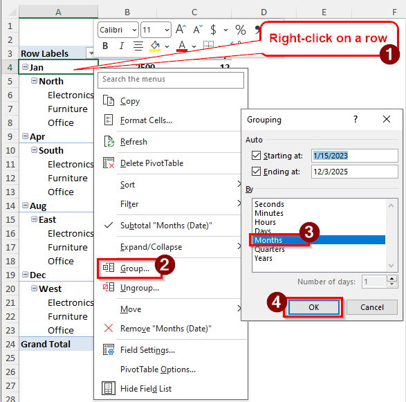
➤ Right-click on a row of the pivot table that has a date value.
➤ Select Group from the context menu.
➤ Deselect anything other than Months. When you have only Months selected, press OK.
Grouping is one of the most essential functions in a pivot table. In this article, we will learn how to group a pivot table by month. We will delve deep and learn everything there is to know about it.
Simple Grouping of Pivot Tables in Excel
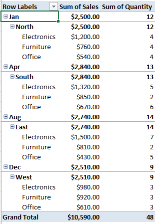
To show how to group by month, we have a dataset with sales data. There is a date, the regions, the category of product, the sales amount, and the quantity of products. The data is from three years, and the sales and quantity count come from four months. However, we want to know the amount of sales for each month regardless of the year. To do that, we have to group the pivot table by month. Follow the steps below to do it:
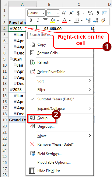
➤ Right-click on a cell that belongs in any row of the pivot table with date values. We are selecting the A4 cell here to do that. After right-clicking, the context menu regarding the field will open.
➤ Select Group from the context menu.
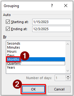
➤ In the new window for Grouping, all of the fields in the Rows area that represent date/time should be selected. We need to keep the Months field selected and unselect the others.
➤ Press OK to confirm the grouping.
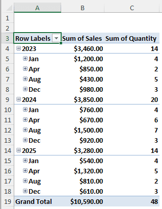
➤ Now the pivot table should be grouped by months.
Creating Advanced Groups in a Pivot Table
The previous method was easy, and it will work if we don’t need to do advanced grouping. However, in data analysis, there is no limitation on what we might have to do. In this method, we will learn how to do advanced grouping by month in a pivot table.
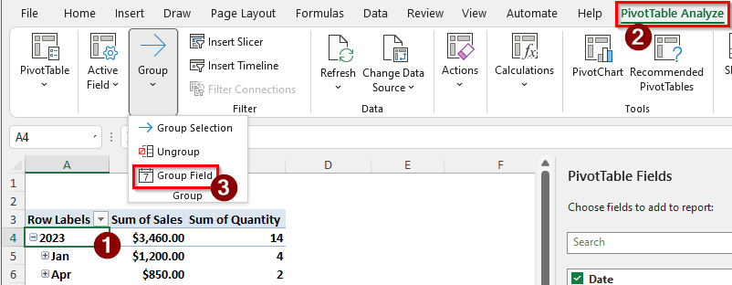
➤ Select a cell containing the date. We are selecting A4 again.
➤ Go to the PivotTable Analyze tab. In the Group section, select Group Field.
➤ Now we can select some advanced options. For example, if we want the values for 2023-2024 only, we will set that date range. Write 1/1/2023 in the Starting at box and 12/31/2024 in the Ending at box. This should also uncheck the Auto boxes, but if it does not, uncheck them manually.
➤ Keep Months selected in the By section and deselect everything else.
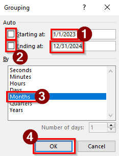
➤Press OK.
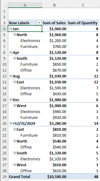
➤ Now, as we can see, the months before 12/31/2024 are shown in a section, and the values after that are shown at the bottom.
Frequently Asked Questions
How do I get pivot tables to stop grouping dates by month?
Pivot table by default groups dates and creates new fields using months, quarters, and years. To stop pivot tables from doing this, go to File > Options from the ribbon at the top. In the new window, select Data. In the right panel, you will find the Data options at the top. From there, check “Disable automatic grouping of Date/Time columns in PivotTables”. Press OK to confirm changes.
How do I filter a pivot table by month instead of day?
In the PivotTable Fields section, find the month field. Then, drag the field and drop it in the Filters section. The pivot table will now have the month filter at the top. You can use the filter from the dropdown context menu of that filter field.
Why are dates not grouping in a pivot table?
Go to the source dataset you used to create the pivot table. Pivot tables are supposed to group the dates automatically. If it’s not doing that, the reason behind that could be that one or more cells in the date column are formatted as text instead of a date. Find those cells in the source dataset and go to Home > Number, and select Date from the dropdown menu. Create a new pivot table to make sure that it groups the dates.
Why is grouping not working in Excel?
There could be several reasons for that. However, data grouping usually does not work when you don’t have the data sorted properly. Sort the data and clear any filters you have for the table. Make sure to convert your range of data to a table by hitting Ctrl + T and clicking OK.
How to use calculated fields in pivot tables?
Select a cell in the pivot table. From the ribbon, go to the PivotTable Analyze tab, and find the Calculations section. Click Fields, Items, & Sets and select Calculated Field. A new window will open that will help you insert a calculated field. Enter the Name of the field and the Formula, then click Add to add the calculated field. Press OK to close the window.
Wrapping Up
In this article, we have learned how to group a pivot table by month. The worksheet used to create and modify the pivot table is available for download. If you have any questions regarding the article or anything related to Excel, please leave them below. We will be back with a new tutorial on a new topic soon.