By grouping the pivot table by week, we can get weekly summaries of our data. If you have some sales data and you want to know the progress of the sales representatives, you would group the weekly data and track sales growth. This article will teach you how to group a pivot table by week in Excel so that you can do the grouping at ease. We will also go through how to choose the starting date, set the week length, set the start and ending date, etc.
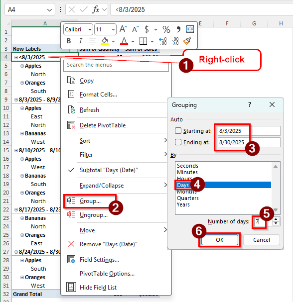
➤ Right-click on a Date value of the pivot table, and select Group.
➤ Change the Starting at date to the start of the first week, and the Ending at date to the end of the last week.
➤ Change By to Days, and write 7 in the Number of days edit box.
➤ Click on OK to do the grouping.
Grouping a pivot table by week is required for a lot of tasks. In this article, we will learn how to do it as efficiently as possible. Therefore, download the Excel file we provided to follow the steps of grouping a pivot table by week with us.
Steps for Grouping a Pivot Table by Week in Excel
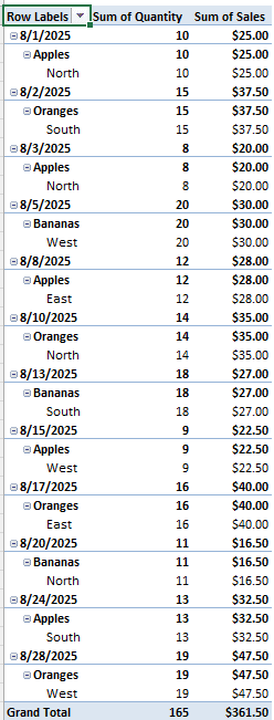
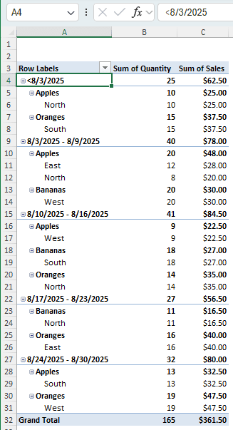
To demonstrate this method, we have a table with sales data. There is a transaction history of a month with product names, regions where they were sold, the quantities, and the sales value. We will group the sales data in the pivot table by week in Excel. Follow the steps below to do so:
Step 1: Head to Grouping Option
To do the grouping, we must go to the pivot table settings, where it allows us to group the pivot table. Here is what you should do:
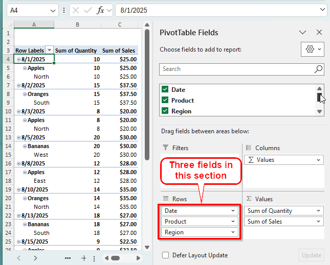
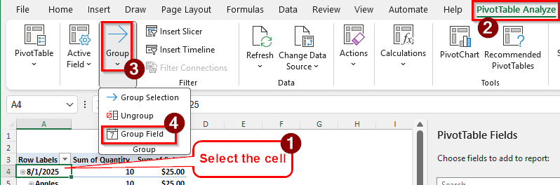
➤ There are three fields in the Rows section. Those are Date, Product, and Region. We will select a cell from the Date field because we want to group using dates.
➤ We can go to the Grouping settings in two ways. First, we can right-click on a cell from “Date”. For example, we can right-click on A4 and select Group from the context menu.
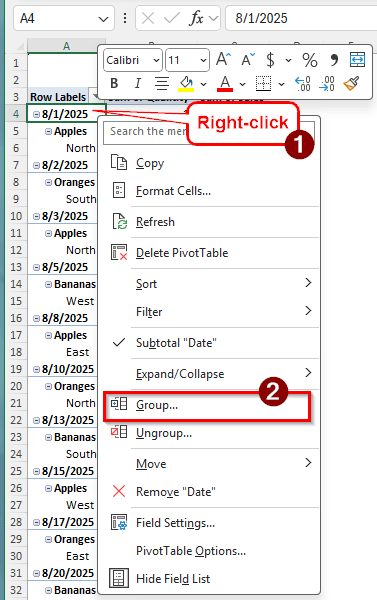
➤ While we are on the A4 cell, we can use the Ribbon to access the window for grouping. There is a tab in the ribbon called PivotTable Analyze. In that tab, there is a section called Group. We can select the Group Field from there to access the Grouping menu.
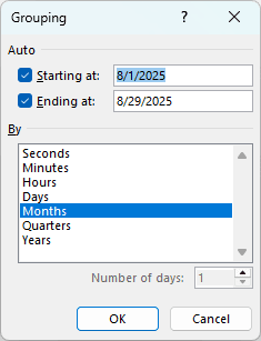
➤ If you follow either of these two methods, a new window will pop up like the following image:
Step 2: Changing the Grouping Options
Now that we have access to the grouping settings, we can change the options and group the pivot table. Follow the instructions below:
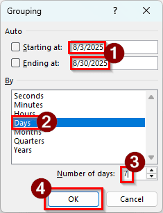
➤ First, we need to change the Starting at date to 8/3/2025 because the first week of August in the year 2025 starts from 8/3/2025, considering that week starts from Sunday. Here is a calendar for reference:
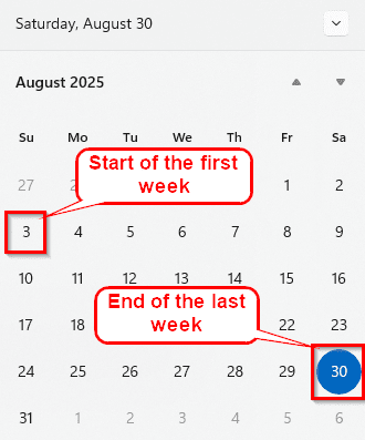
➤ Next, we change the Ending at date to 8/30/2025 because that marks the end of the last week of the month.
➤ In the By section, we select Days only. Months are already selected here, but we can click on that to deselect them. Then, change the Number of days to 7.
Note:
When changing the Starting at & Ending at dates, the checkboxes on the left should automatically be unchecked. If they are not, please manually uncheck them.
➤ Press OK to confirm and see changes in the pivot table.
Frequently Asked Questions
How to create a week filter in a pivot table?
There are basically two ways to do this. If you already have the weeks mentioned in your dataset, you can use that field in the Filters area of the PivotTable Fields to create a filter. If you don’t have the weeks, you can create a calculated field or add one in the source data, then use that field in the Filters area. Just drag and drop the field in that area, and a new dropdown will be created at the top of the pivot table. You can use that dropdown to select the filter.
How to use Weeknum?
The WEEKNUM function in Excel returns the week number in a cell. It takes one required parameter and one optional parameter. The required parameter is the date. For example, if we enter 8/1/2025 in this parameter, the function will return 31 because that day belongs to the 31st week of the year. Look at the example below:
=WEEKNUM(8/1/2025)
The optional parameter is used to specify the day when the week starts. We don’t need to put that here because it assumes the starting day is Sunday in the US.
How to calculate weeks per month?
First, count the days of the month. A month can have 28 to 31 days. Then, divide the days by 7, as there are 7 days in a week. For example, February has 28 days in general. Divided by 7, there are four weeks in February. Most months will have more than 4 weeks, and you will get a decimal number instead.
How to filter by month in a pivot table?
Click on the dropdown of the Row Labels cell of the pivot table. In that menu, you can find different filtering options. An option should be called “Date Filters”. There would be a lot of options to filter by dates in the submenu of Date Filters. Select the month filter that you want to try.
What is the difference between weekday and weeknum?
Both WEEKDAY and WEEKNUM are useful functions in Microsoft Excel. Both functions require one parameter, which is the date. However, the output from these functions varies. For the first function, the output is the number of the day of the week. The second function returns the number of the week in the whole year.
Wrapping Up
In this article, we have learned how to group a pivot table by week. We hope that the step-by-step guide provided in this article helped you learn how to use the group function of a pivot table. If you have some other methods that you believe will be better for the task, leave them in the comments section. We would love to check those out. Stay tuned for more Excel tutorials.