Using slicers is a super-easy way to filter data in a pivot table. Even if you don’t know any formulas, functions, or other Excel tools, you can use slicers to easily filter your data visually with almost no drawbacks. In this article, we will learn how to insert slicer in excel with pivot table.
➤ Select any cell of the pivot table to enable PivotTable Analyze and Design
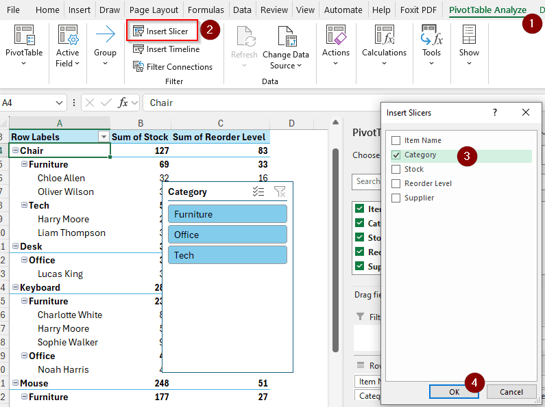
➤ Go to PivotTable Analyze tab and click on Insert Slicer from the Filter
➤ Select the fields you want to insert slicers for and click OK.
Now you know how to insert a slicer, but this tutorial offers you more. We will go in-depth on how to insert and use a slicer in pivot tables. Therefore, stick around and read the full article to be a pro on using slicers.
Inserting Slicer in Excel with Pivot Table
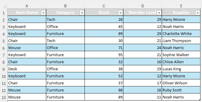
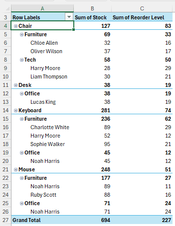
Here, we have some product stock information. The items, stock and reorder levels, categories of where the product should go, and supplier names. We can use a lot of filters on this data, but first, we need to add slicers in the pivot table to do so.
Follow the steps below to do it:
Step 1: Creating a Pivot Table
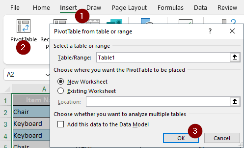
➤ Select the data range/table and go to Insert > PivotTable
➤ Keep the options as it is and click OK to place the new pivot table in a new worksheet
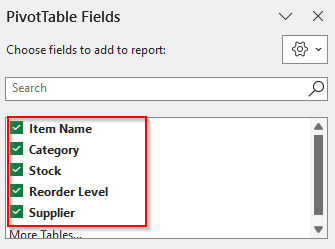
➤ In the new worksheet, select all of the fields from the PivotTable Fields panel on the right.
➤ Now the pivot table sheet should look like this:
Step 2: Adding Slicers
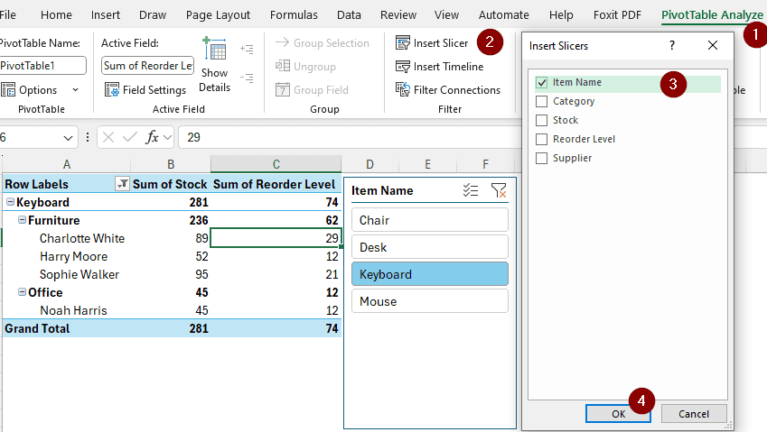
➤ When you have any of the cells of the pivot table selected, go to the PivotTable Analyze tab
➤ Click on the Insert Slicer button in the Filter section.
➤ Now choose the columns you want to filter your data from and Press OK
Using Slicers in Excel
Inserting a slicer is of no use if you don’t know how to use slicer in Excel. For your convenience, here are some uses of slicers that will help you for sure.
Working with Filters
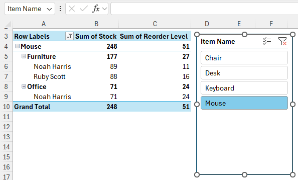
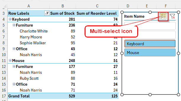
➤ In our current slicer, “Item Name”, we can select individual items to display entries about those specific In the beginning, every item is shown. Here, we are selecting Mouse to show entries with Mouse only.
➤ We can select multiple items by holding Ctrl while selecting. We can also select multiple items by enabling the Multi-Select Icon at the top. That Icon can also be enabled by pressing Alt + S .
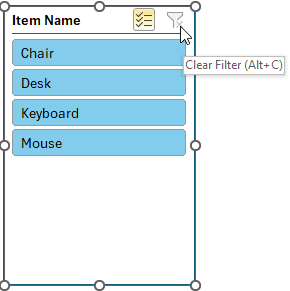
➤ We can clear our selection by clicking the Clear Filter icon at the top right, or by pressing Alt + C .
Designing the Slicer
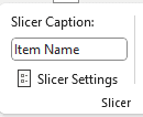
➤ From the Slicer tab, go to the “Slicer Caption:” option to change the caption of the slicer.
➤ You can go to Slicer Styles from the same tab to change the whole design of the slicer
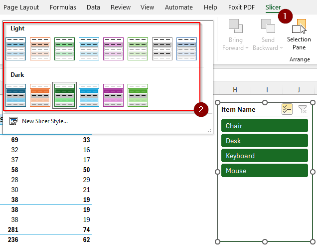
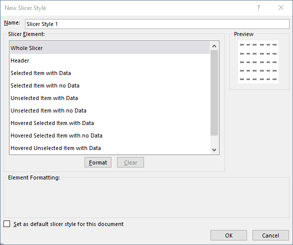
➤ By hitting New Slicer Style, you can create your own style for the slicer. Change the name, edit different elements of the slicer, and hit OK.
Frequently Asked Questions
How to insert slicer in Excel without PivotTable?
First, convert your dataset to a table by pressing Ctrl + T . Then, go to the Table Design tab, and hit Insert Slicer from the Tools section. Now you can add a slicer according to your choice.
How do I link a PivotTable to one slicer?
Click on the slicer to enable the Slicer tab. From the left side of the tab, select Report Connections. From the new window, select the pivot tables you want to link to that slicer.
Do Excel slicers only work with pivot tables?
No. Excel slicers work with pivot tables, regular tables, and pivot charts. However, if you are using an older version of Excel, you might not be able to use slicers in anything other than pivot tables.
Why won’t my slicer connect to all pivot tables?
If your slicer is not connecting to all pivot tables nor showing the connections, you need to recreate the pivot tables with the same source of data. When the pivot tables are from different sources, slicers cannot connect to them as it is not possible to filter with fully separate connections.
How do I add a filter to a pivot table?
When the PivotTable Fields panel is enabled, drag the desired field from the columns/rows/values area to the Filters area using your mouse. In the spreadsheet, you can now locate the filter at the top.
Wrapping Up
In this article, we have learned how to insert a slicer in Excel with a pivot table properly. We have also learned how to use slicers in a pivot table so that you can make use of the tool for your dataset. Download the sample dataset for practice, and leave a comment below with your suggestions.