While using pivot tables, we often have to check text data as values. These data are shown as a count in the pivot table, as there is nothing to sum up. Imagine you have an office, and there is an employee list depending on the departments they work in.
In order to count the employees of the different departments and the number of employees in the whole office, you will need to use count. And to know which departments have the most or least employees, you will have to sort the pivot table by count. In this article, we will learn how to sort a pivot table by count.
➤ Click on the small arrow on the bottom-right of the cell that says “Row Labels” in the pivot table.
➤ Select More Options.
➤ In the new window, select Descending (Z to A) to sort from largest to smallest, and Ascending (A to Z) to sort from smallest to largest.
➤ From the dropdown menu next to the sorting option, select the value that includes the Count. Press OK to confirm.
Sorting is one of the most important and useful functions of data analysis. Pivot tables allow you to sort your data in many ways, no matter how the data values are formatted. Here are three ways you can sort your pivot table by count.
Sorting from More Sort Options
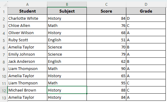
We are using a dataset with some student names, the subjects they are enrolled in, their scores, and grades. We want to know how many students are enrolled in each subject, then sort the pivot table according to the count of students to know which subject has the most students. Here is the dataset:
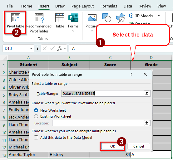
➤ Select A1:D13 cells of the dataset and go to the Insert tab from the Ribbon at the top.
➤ Click on PivotTable from the Tables section of that tab.
➤ We don’t need to change anything in the new window that popped up. Click OK to create the pivot table in another sheet.
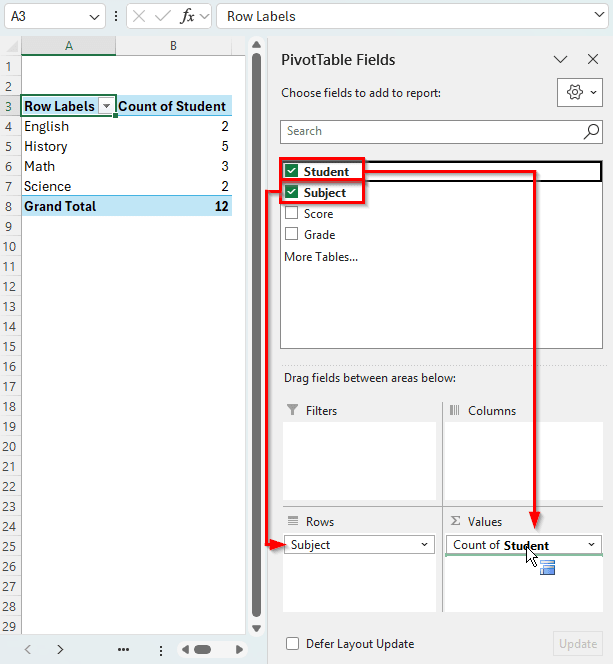
➤ In the PivotTable Fields section, drag and drop the Subject in the Rows section, and the Student to the Values section. As there are no numerical values in the Student column, Excel should automatically use Count for calculation.
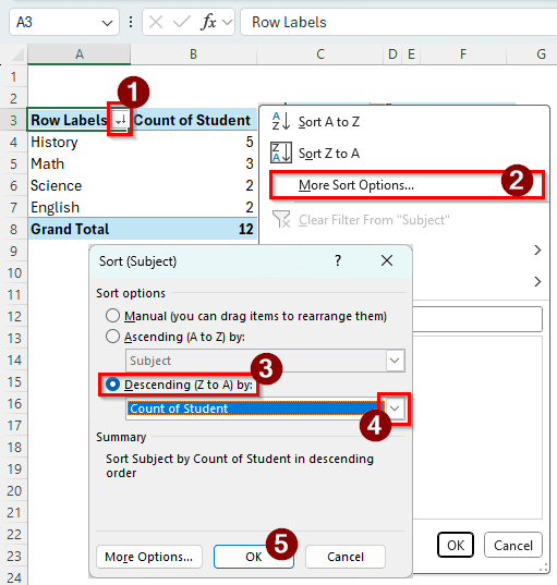
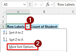
➤ Click on the small arrow that is facing downwards on the A3 cell.
➤ Select More Sort Options.
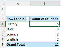
➤ Select “Descending (Z to A) by” radio button. Then, from the dropdown menu, select “Count of Student”
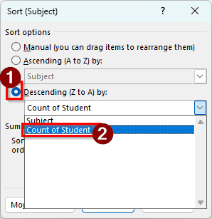
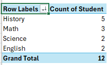
➤ Press OK to see the result.
Sorting from the Ribbon
There are two ways to sort using the Ribbon in Microsoft Excel. Read the instructions below to learn the ways.
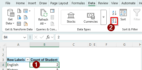
➤ Click on the B4 cell of the pivot table. You can select any cell from B4:B7 as long as they are of the “Count of Student”
➤ Go to the Data tab and find the Sort & Filter section. There should be three buttons on the left side. Click on “Sort Largest to Smallest” to do so.
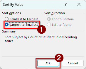
➤ You can also click on the Sort button to open a new window for sorting. Select Largest to Smallest and hit OK to confirm.
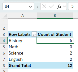
➤ Finally, the table should look like the following:
Sorting from Context Menu
This is the easiest method to sort the pivot table by count. Here is how to do it:
➤ Select a cell from the range B4:B7.
➤ Right-click on that cell to open the context menu.
➤ Go to Sort > Sort Largest to Smallest.
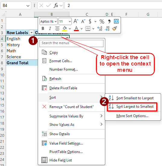
➤ That’s it, the table is now sorted from largest to smallest. You can select Sort Smallest to Largest to do the opposite.
Frequently Asked Questions
How to do a PivotTable with count?
If your data has numbers, Excel will usually make the pivot table show the sum of those values. To change it to count, click on the field from the Values section of the PivotTable Fields section. Select the Value Field Settings to open a new window. From that window, select Count from the “Summarize Values By” tab. Click OK to confirm.
How to sort a PivotTable by total value?
Click on a total value in the pivot table. It can be the grand total or the subtotal, depending on what you want. Then right-click on the cell, and move your mouse to Sort to open the sorting options. Select “Sort Smallest to Largest” or “Sort Largest to Smallest” based on your preference.
How to collapse all in an Excel PivotTable?
Right-click on the field that you want to collapse every cell of. Go to Expand/Collapse from the context menu, and select Collapse Entire Field. All of the fields in the same row category will be collapsed. If you want to collapse the whole pivot table, select the topmost row for right-clicking.
Why is my PivotTable not counting correctly?
Go to the source dataset and find the cells that are not counted properly in the pivot table. Click on the cell and select Number from the dropdown menu in the Number section of the Home tab. Go back to the pivot table, and refresh the table by right-clicking on any cell of the table and hitting Refresh. Your pivot table should count correctly now.
Why is the sort range greyed out?
Microsoft Excel allows the user to protect the worksheet. If you got the worksheet from someone else, it might be protected to prevent editing. In case you downloaded the file from the Internet, chances are Microsoft has enabled protected mode to protect you from potential dangers. You can enable editing to sort the ranges.
Wrapping Up
In this article, we have learned how to sort a pivot table by count. We hope you have grasped all three methods mentioned in this article. In case you have issues with following the instructions, leave a comment below so that we can help you out. Bookmark the website so that you can get back for more Excel tutorials.