Pivot Tables are used for data summarization in Excel, but presenting the data in a sorted order is just as important as calculating it. A common need is to sort the Pivot Table rows or columns based on the sum of their values, such as identifying the top-selling products or the highest-performing month. While Excel’s sorting feature is straightforward for alphabetical order, sorting by a cumulative sum requires specific techniques. In this article, we will guide you through two methods to sort Pivot Table by sum of values.
To sort Pivot Table data by the sum of values, here is one simple solution by using the Sort feature in Excel.
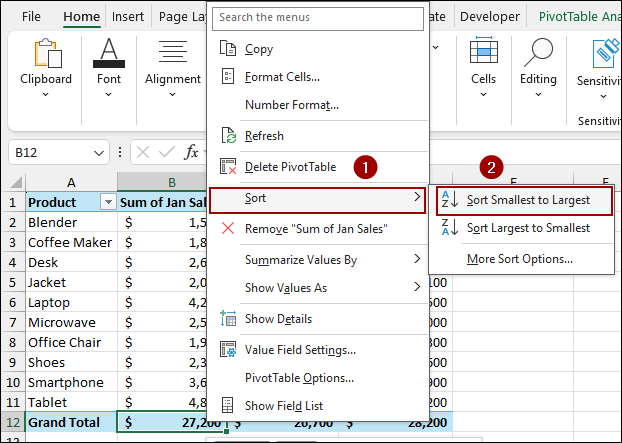
➤ Right-click the Grand Total cell for the columns you want to sort.
➤ Click Sort > Sort Smallest to Largest to get the Pivot Table sorted by sum of values.
Using Sort Feature to Sort Horizontally
If you have multiple data columns (like different months) and want to sort the columns based on their sum of values (e.g., arrange months from lowest total sales to highest total sales), you can use the built-in Sort option.
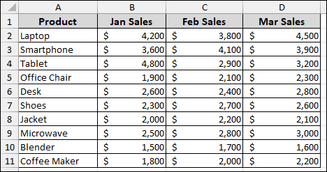
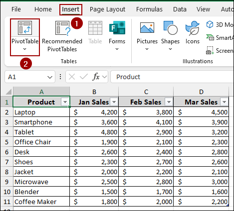
Imagine a sample dataset showing monthly sales figures for several products. Here, we will convert the data range into a PivotTable and then use the Sort feature to sort by the sum of values.
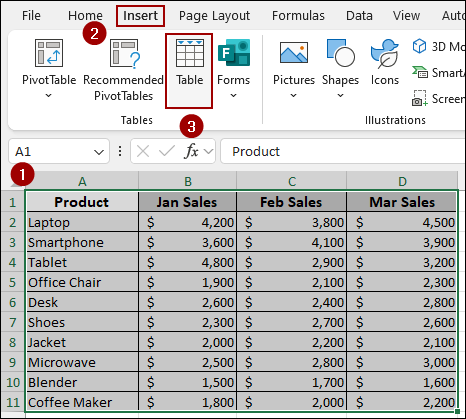
To convert data into an Excel Table.
➤ Select the dataset (A1:D11).
➤ Go to the Insert tab, click Table.
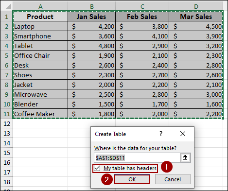
➤ Checkmark My table has headers and click OK.
Now, the data range will be converted into a Table. To create a Pivot Table:
➤ Go to the Insert tab, click PivotTable.
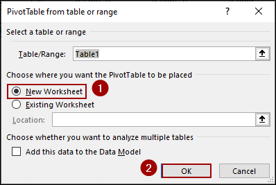
➤ Select New Worksheet, and click OK.
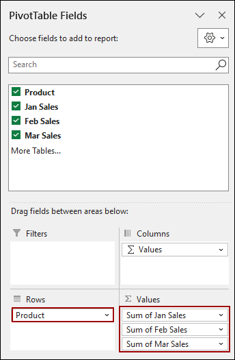
For horizontal sorting, ensure your months are in the Values area and your products are in the Rows area.
➤ Drag the Product field to the Rows area.
➤ Drag Jan Sales, Feb Sales, and Mar Sales fields to the Values area.
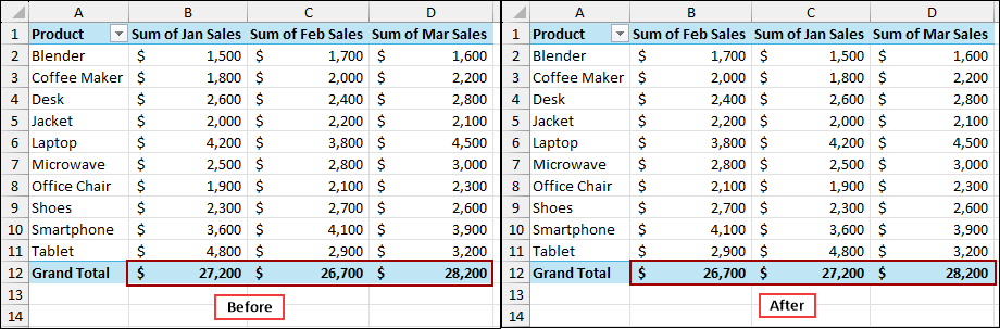
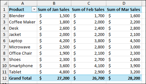
The initial Pivot Table is created, showing the sum of sales for each month. Notice the months are currently ordered Jan, Feb, Mar with Grand Totals of 27,200, 26,700, and 28,200, respectively.
To sort the month columns by their total sales (the Grand Total row):
➤ Right-click on the Grand Total cell for the first month (Sum of Jan Sales, cell B12).
➤ Hover over Sort and choose Sort Smallest to Largest to rearrange the months based on their total sales.
The Pivot Table columns are now sorted based on the month with the smallest total sales (Feb Sales) to the largest (Mar Sales).

Applying Calculated Field to Sort Vertically
Sorting the row items (like products) by the sum of their values (e.g., sorting products by their total three-month sales) requires a slightly different approach. Here, we will use the Calculated Field feature to sum sales and then use the Sort tool.
We need a single column that represents the total sales across all months for each product.
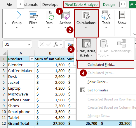
➤ Click inside your Pivot Table.
➤ Navigate to the PivotTable Analyze tab.
➤ In the Calculations group, click on Fields, Items, & Sets.
➤ Select Calculated Field.
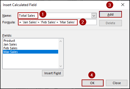
In the Insert Calculated Field dialog box:
➤ In the Name box, type Total Sales.
➤ In the Formula box, enter the sum of the monthly sales fields.
='Jan Sales' + 'Feb Sales' + 'Mar Sales'
You can double-click the field names in the list to insert them.
➤ Click Add and then OK.
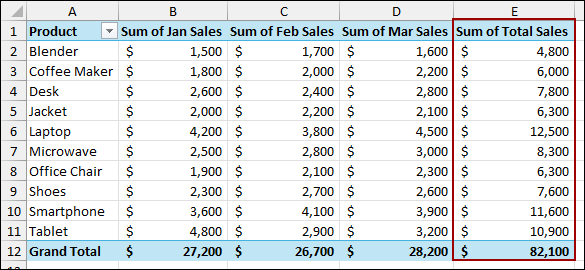
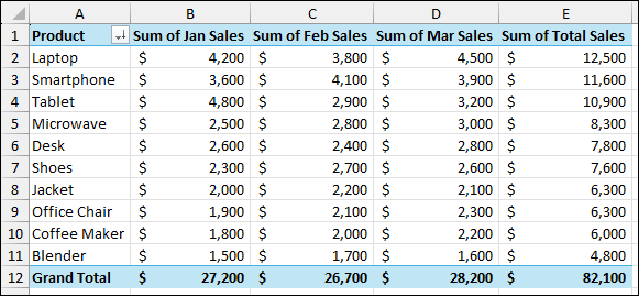
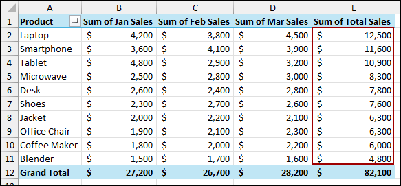
A new column, Sum of Total Sales, added to the Pivot Table, displaying the three-month sum for each product.
With the Sum of Total Sales column now present, we will sort the Product row field based on its values.
➤ Right-click on any value in the new Sum of Total Sales column (e.g., cell E2).
➤ Hover over Sort and choose Sort Largest to Smallest.
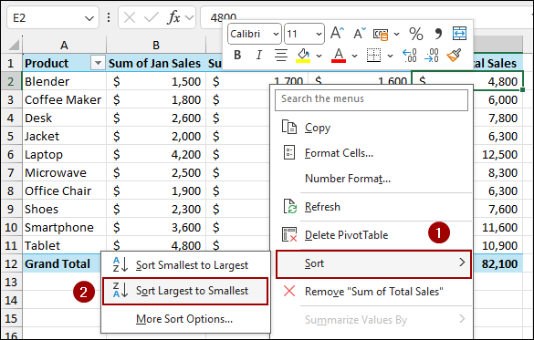
The products are now successfully sorted from the highest total sales (Laptop with $12,500) to the lowest (Blender with $4,800).
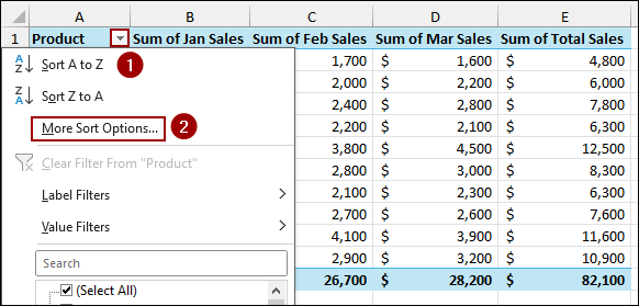
Alternatively, we can use the More Sort Options dialog box.
➤ Click the dropdown Arrow next to the Product field in cell A1.
➤ Select More Sort Options.
In the Sort (Product) dialog box:
➤ Select Descending (Z to A) by.
➤ From the dropdown menu, choose Sum of Total Sales.
➤ Click OK.
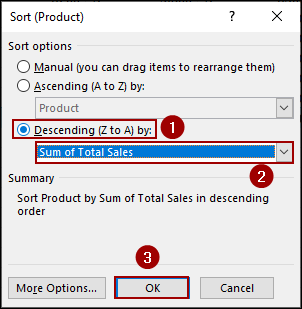
As a result, we will get the same output where the Pivot Table is sorted vertically by the total sum of the values.
Frequently Asked Questions
Why is my PivotTable not sorting by the correct sum of values?
This usually happens if the field is summarized by Count instead of Sum. Check Field Settings and change it to Sum before sorting.
My PivotTable sort order keeps resetting when I refresh. How do I fix this?
PivotTables sometimes revert to default order after refresh. To fix, reapply the sort or use a Custom List so that your chosen order is preserved.
Can I manually rearrange items instead of sorting by values?
Yes. You can drag and drop row/column labels directly inside the PivotTable for a manual custom order.
Concluding Words
Above, we have explored two essential methods for sorting Pivot Table data by the sum of its values. For quick comparison and sorting Pivot Table horizontally, use the Sort tool on the grand total row. For more effective ordering based on a cumulative total, the Calculated Field feature provides the necessary sorting key. If you have any questions, please don’t hesitate to share them in the comments section below.