Marking the blank cells in your worksheet helps you avoid issues with data analysis, project tracking, spotting errors, and accidentally removing data. While there are many static and dynamic ways of finding and highlighting blank cells, applying Conditional Formatting rules is the most effective way.
It allows you to format blank cells with a fill color to instantly find an empty cell among thousands of used cells.
Steps to use Conditional Formatting to find and highlight blanks:
➤ Select your data range (or press Ctrl + A to select the entire sheet) and go to the Home tab. Select Conditional Formatting >> New Rule.
➤ From the Select a Rule Type group, choose Format Only Cells That Contain.
➤ Click on the Format Only Cells With drop-down and select Blanks. Click on Format.
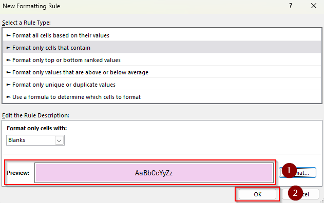
➤ Choose a fill color from the Fill tab and click Ok. Preview the formatting and press Ok.
Apart from this effective method, we’ll cover more ways to find and highlight blank cells using the Go To Special feature, Find & Replace tool, Conditional Formatting with a formula, and VBA coding.
Manually Highlight Blank Cells
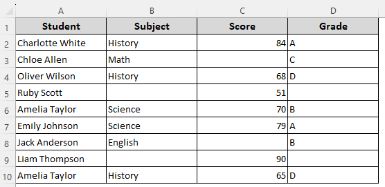
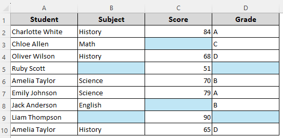
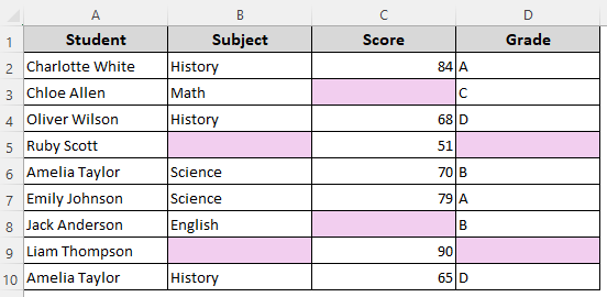
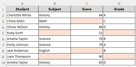
Our sample dataset contains columns for student names, different subjects, and their attained marks. Here, the cells B5, B9, C3, C8, D5, and D9 are blank. We’ll find those cells and highlight them with a background color.
For only a few blank cells in a small dataset, you can locate the blank cells, select them manually, and highlight them with a fill color. This method isn’t suitable for large datasets with a huge number of empty cells. Here are the details:
➤ Select the first blank cell and press the Ctrl button on your keyboard. Hold it as you manually select all the remaining blank cells
![]()
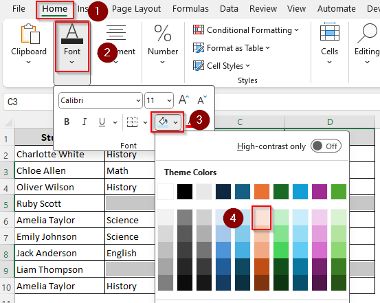
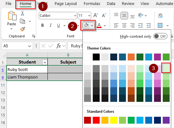
➤ Once all the blanks are selected, open the Home tab and click on the Fill Color drop-down (paint color icon) in the Font group.
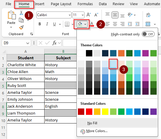
➤ Select a color to set it as a background color to highlight the blank cells.
Find and Highlight Blank Cells with the Go To Special Feature
With Excel’s Go To Special feature, you can select all the blank cells at once. Later, we’ll use a fill color to highlight them. Keep in mind that this method is for truly blank cells.
If the cell is visibly empty but contains an empty string, a space, or other non-printable characters, it won’t be highlighted. Also, the changes are static, so newly added blanks won’t be highlighted automatically. Below are the steps:
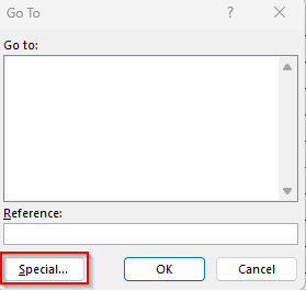
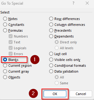
➤ Select your data range and press Ctrl + G . From the Go To box, click on Special.
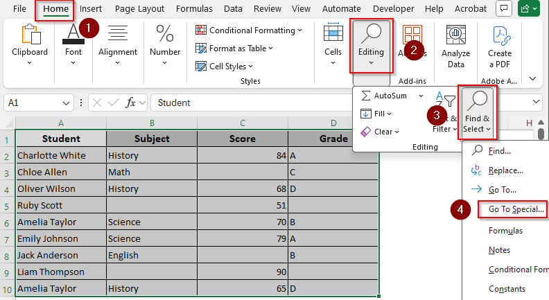
➤ Or, go to the Home tab >> Editing >> Find & Select >> Go To Special.
➤ In the Go To Special dialog box, click on Blanks and press Ok to highlight all the blank cells.
➤ From the Home tab, press the Fill Color icon from the Font group. Choose a color to highlight the selected cells.
➤ Here’s the final result:
![]()
Locate and Highlight Blank Cells with the Find & Replace Tool
Similar to the previous method, this also selects all blank cells at once. The Find & Replace tool will find only the truly blank cells in your worksheet. Here’s how:
➤ Select your range and press Ctrl + F . You can also go to the Home tab >> Editing >> Find & Select >> Replace.
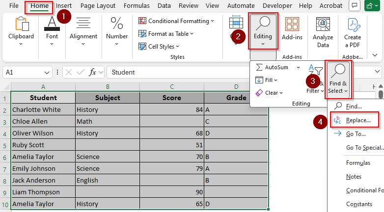
➤ As the Find and Replace dialog box opens, leave the Find What field completely empty. Click on Options to expand advanced options.
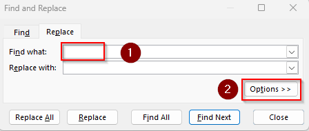
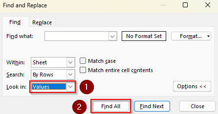
➤ In the Look In dropdown, choose Values. Click Find All.
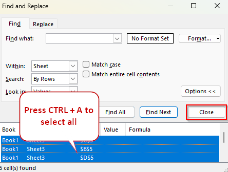
➤ Excel will list all blank cells found in the selected range. To select them all at once, click inside the results box and press Ctrl + A . Press Close.
➤ Finally, go to the Home tab, click on the Fill Color icon, and select a color to highlight the blank cells permanently.
➤ The result for our dataset is as follows:
Set Conditional Formatting Rules to Find and Highlight Blanks
Applying a Conditional Formatting rule is a dynamic solution to highlight blank cells even for new entries. We’ll set a new formatting rule for the empty cells and select our preferred format to highlight them.
With this method, you can select truly blank cells and zero-length strings or empty strings. For this, follow the steps given below:
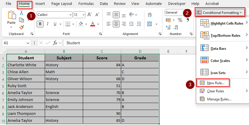
➤ Select your data range and go to the Home tab.
➤ From the Styles group, click on Conditional Formatting. Choose New Rule from the drop-down menu.
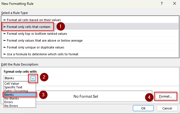
➤ As the New Formatting Rule dialog box appears, select Format Only Cells That Contain from the Select a Rule Type group.
➤ Click on the Format Only Cells With drop-down and choose Blanks.

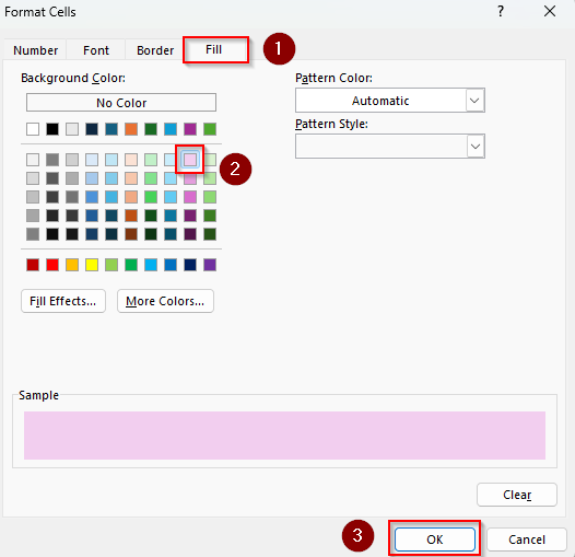
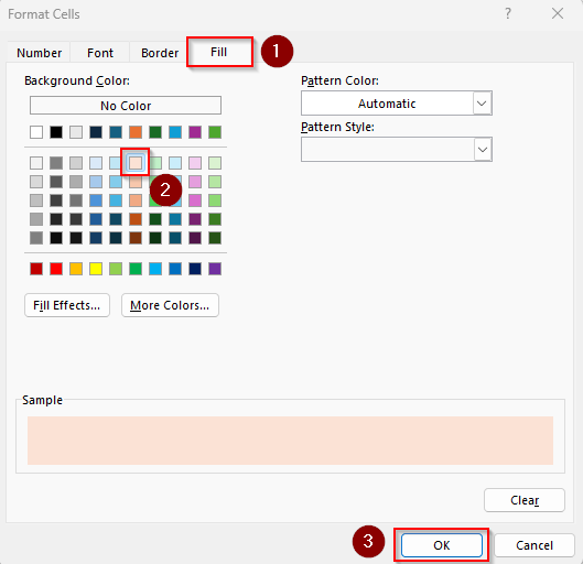
➤ Now, press the Format button and select the Fill tab. Choose a color from the Background Color group and click Ok.
➤ Finally, check the Preview section to see how the highlighted cells will be formatted. Press Ok.
➤ Let’s take a look at the final result for our dataset:
Apply Conditional Formatting Rules with a Formula to Highlight Empty Cells
Another way to highlight blank cells is to apply a formula using the Conditional Formatting feature. You can use a formula for truly blank cells or cells with empty strings. Below are the steps:
➤ Select your data range and click on the Home tab >> Conditional Formatting >> New Rule.

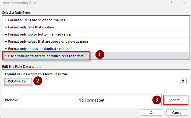
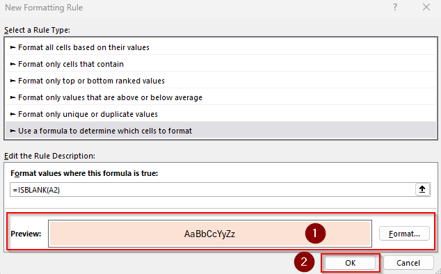
➤ From the Select a Rule Type group, choose Use a Formula to Determine Which Cells to Format.
➤ In the Format Values Where This Formula Is True box, enter any of the following formulas:
For Truly Blank Cells
=ISBLANK(A2)
For Blank Cells and Empty Strings
=LEN(A2)=0
➤ In both formulas, A2 is the top-left cell (first cell) of your selection. Change it according to your dataset.
➤ Click on Format >> Fill tab. Choose a background color and click Ok.
➤ Check the Preview box and press Ok.
➤ Here’s the final result:
Use a Filter to Find and Highlight Rows with Blank Cells
If you want to highlight the entire row containing one or more blank cells, you can use the Filter feature. As it filters the rows with blank cells, we can use a fill color to highlight them.
However, this method works only on a single column at a time. Therefore, you need to repeat it for each column with blanks. Let’s get to the steps:
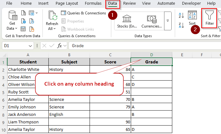
➤ Click on any column heading and go to the Data tab. Select Filter from the Sort & Filter group.
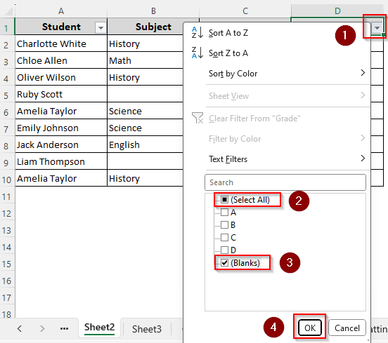
➤ Select the column with blank cells and click the Filter drop-down on the column heading.
➤ Uncheck Select All and check Blanks. Press Ok.
➤ As Excel lists all the rows with blank cells, select them all excluding the header row.
➤ Go to the Home tab, click on the Fill Color icon, and select a background color.
➤ To remove the filter, go to the Data tab >> Filter. This will bring back the remaining cells with highlighted rows. Repeat the steps for other columns.
![]()
Find and Highlight Blanks with a Custom VBA Macro
In this method, we’ll code a custom VBA macro to effectively highlight all blank cells in your worksheet. Here are the steps:
➤ To add the Developer tab in your main ribbon, go to the File tab >> More >> Options.
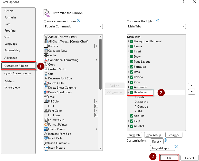
➤ Click on Customize Ribbon and check the Developer box. Press Ok.
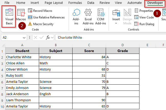
➤ Now, open the Developer tab and click on Visual Basic.
➤ In the VBA Editor, select the Insert tab >> Module.
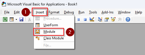
➤ Paste the following code in the blank Module box:
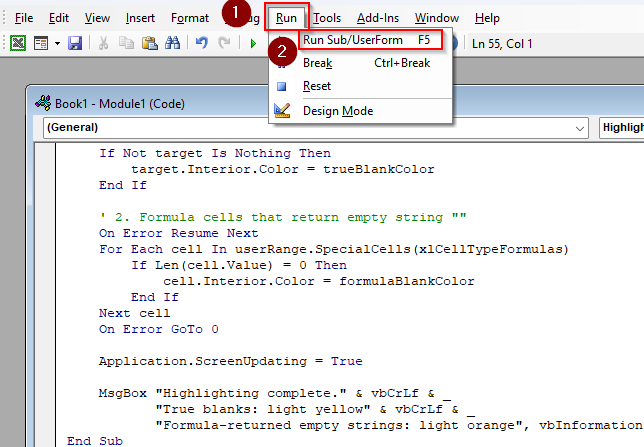
➤ Press F5 to run the macro or click on Run >> Run Sub/UserForm.
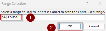
➤ As Excel prompts you to select a range to find blank cells from, manually type the range or go back to the Excel tab and highlight the range and click Ok. Or, press Cancel to select the entire used range.
➤ All the blank cells are now highlighted.
![]()
Frequently Asked Questions
How to find blank cells in Excel and fill?
Select your data range, press Ctrl + G , and click Special. Choose Blanks from the given options and press Ok. With the blank cells selected, type a value such as 0, N/A, or a formula. Press Ctrl + Enter to fill all selected blanks at once with the same value you typed.
How to select only filled cells in Excel?
Click on the header row and go to the Data tab >> Filter. Choose any column heading and click the Filter dropdown. Uncheck Blanks to highlight only filled rows.
How to identify blank columns in Excel?
In a new helper row, insert this formula:
=COUNTA(A1:A10)
Change the column range (A1:A10) according to your dataset. Press Enter and drag the formula across all columns. Columns showing 0 are completely blank.
Concluding Words
Highlighting blank cells with a background marks them permanently. Depending on whether you want to automatically mark blank cells for future entries or not, choose a dynamic or static method. If you want to undo the changes, repeat the steps for each method and click on the Home tab >> Fill Color icon. Now, choose No Fill from the color palette.