When a formula returns an error, zero, or negative numbers, you might want to replace it with a blank instead for a cleaner look. Although Excel doesn’t allow a formula to truly delete a cell’s contents, you can make it appear empty by replacing its value with an empty string (“”).
It’s useful for creating analytical reports, hiding zero values, or making logic easier to follow. Using the IF function is the best way to return an empty string based on a condition.
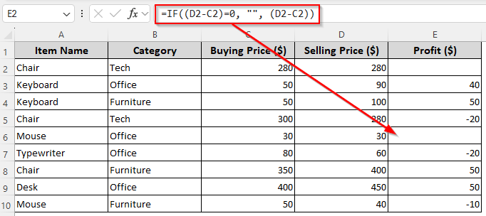
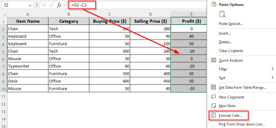
➤ Let’s say we have the buying price of a product in C2 and its selling price in D2. To calculate the profit and replace a returned zero (0) with an empty string, use the IF function as shown in the following formula:
=IF((D2-C2)=0, “”, (D2-C2))
➤ You can replace the formula (D2-C2) and cell references according to your dataset.
➤ Press Enter and drag the formula down to apply the same condition to the remaining cells.
This article covers all the ways of setting a cell to blank in a formula using functions like the IF, ISBLANK, IFERROR, OR, AND, and VBA coding.
Using the IF Function to Set a Cell to Blank in a Formula
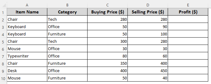
Our sample dataset contains product names, their buying and selling prices, and other info. We’ll use the buying prices in column C and the selling prices in column D to apply various formulas. Based on the formula result, we’ll set blank cells in column E.
In Excel, the IF function checks if a condition is true or false and returns one value if the condition is true and another value if the condition is false. So, we can combine it with other formulas and set conditions to return an empty string for certain results such as a zero or negative number. Here’s how to use it:
➤ In a column where you want to return the blanks, enter any of the following formulas:
Set Blank If Formula Returns a Zero
➤ To make a formula return an empty string instead of a zero, use the IF function as shown below:
=IF((D2-C2)=0, "", (D2-C2))
➤ Instead of (D2-C2), you can use any other formula with the same syntax. Replace the cell references as needed.
➤ Press Enter. Use the fill handle (+ sign on the bottom corner of a cell) to autofill the remaining cells.

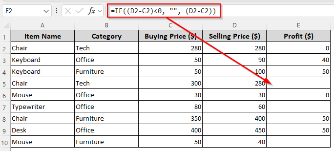
Set Blank If Formula Returns Negative Value
➤ For replacing negative values with blanks, use the following formula:
=IF((D2-C2)<0, "", (D2-C2))
➤ Replace (D2-C2) with any other formula and change the cell references as needed.
➤ Click Enter and drag the formula down using the fill handle.
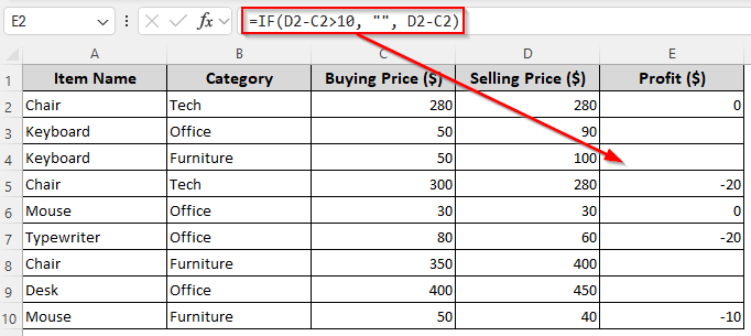
Set Blank for Less/Greater Than Conditions
➤ If you want to make a formula return a blank if the formula result is less than 10, enter this formula:
=IF(D2-C2>10, "", D2-C2)
➤ Change the formula and cell references according to your dataset.
➤ Press Enter and drag the formula down to fill the remaining cells.
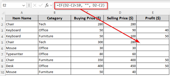
➤ To return blanks for values greater than 10, use this formula, press Enter, and drag it down:
=IF(D2-C2<10, "", D2-C2)
Returning Blanks for Formula Errors with the IFERROR and IFNA Functions
When a formula might return an error and you want to display a blank instead, use the IFERROR or IFNA functions. Here’s how:
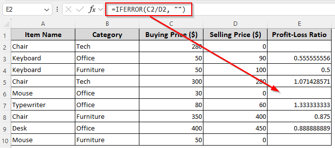
For All Types of Errors
➤ Dividing a value with zero(0) gives you a #DIV/0! error. To avoid this, use the IFERROR function in the following way:
=IFERROR(C2/D2, "")
➤ Change the formula C2/D2 and cell references as per your dataset.
➤ Press Enter and drag the formula down.
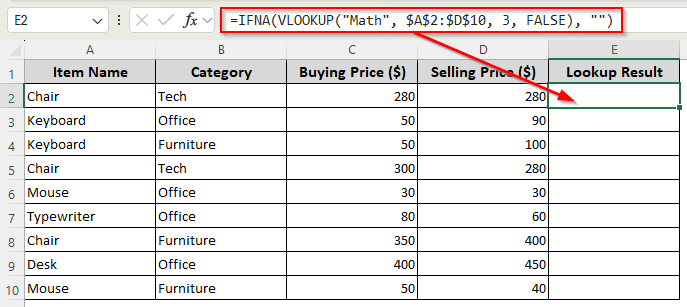
For #N/A Errors Only
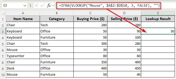
Usually, when a lookup function (like VLOOKUP, HLOOKUP, or MATCH) can’t find the specified value within the lookup range, it returns a #N/A error. So, we’ll look for the value Math in our data range $A$2:$D$10.
If found, we want the formula to return the corresponding value from the 3rd column (column C). Otherwise, it should return an empty string. As we don’t have the text Math in our dataset, the formula returns an empty string instead of a #N/A error. Below are the details:
➤ Insert the following formula:
=IFNA(VLOOKUP("Math", $A$2:$D$10, 3, FALSE), "")
➤ Change the lookup value, range, and column number according to your dataset. Click Enter.
➤ On the other hand, if we look for the value Mouse, Excel returns the correct value from column C as shown below:
=IFNA(VLOOKUP("Mouse", $A$2:$D$10, 3, FALSE), "")
Return a Blank for Formula Using the IF and ISBLANK Functions
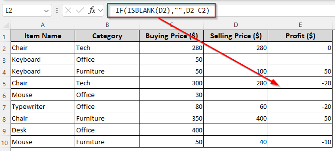
If you want a cell to remain blank based on another cell’s blank status, use the IF and ISBLANK functions. The ISBLANK function checks if a cell is blank or contains data.
Combining it with the IF function allows you to make a formula to avoid working on blank cells and return an empty string. Below are the steps to use the two functions:
➤ To make a formula not count blank cells, type the following formula:
=IF(ISBLANK(D2),"",D2-C2)
➤ This formula checks if D2 is empty. If yes, it returns blank. Otherwise, it subtracts the value of D2 from C2.
➤ Here, D2 is the first cell of the column containing several blank cells. Change the cell reference and formula D2-C2 as required.
➤ Press Enter and use the fill handle to autofill the rest of the cells.
Combining the IF and OR/AND Functions to Return Blanks Based on Multiple Conditions
You can combine multiple conditions using the IF and OR/AND functions. If one or both conditions are met, the formula will return a blank. Follow the steps given below:
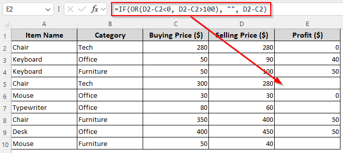
Set Blank If At Least One Condition Is Met
➤ If the result of our subtraction formula is less than 0 or greater than 100, the following formula will return an empty string:
=IF(OR(D2-C2<0, D2-C2>100), "", D2-C2)
➤ Change the conditions, formula, and cell references according to your dataset.
➤ Click Enter and drag the formula down.
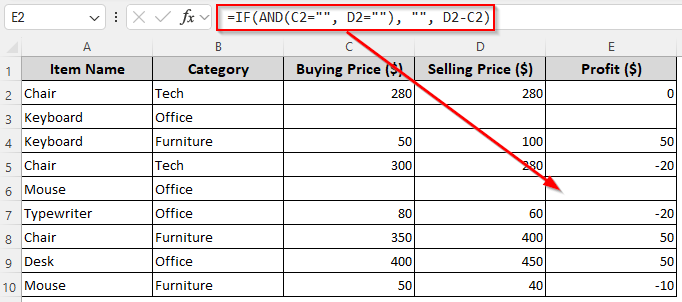
Set Blank If Both Conditions Are Met
➤ The following formula returns an empty string if both C2 and D2 are blank:
=IF(AND(C2="", D2=""), "", D2-C2)
➤ Replace the conditions, formulas, and cell references as required.
➤ Press Enter and autofill the remaining cells using the fill handle.
Convert Zeros to Blank Using Custom Cell Formatting
As a formula returns zero, you can replace it with a blank using the Format Cells option. Here’s how:
➤ Select the cells or cell range containing the zeros you want to convert and press Ctrl + 1 .
➤ Or, right-click on your selection and choose Format Cells from the menu.
➤ Click on the Number tab and select Custom from the Category group.
➤ In the Type field, insert the format given below:
0;-0;;@
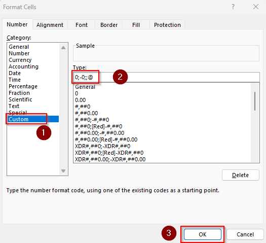
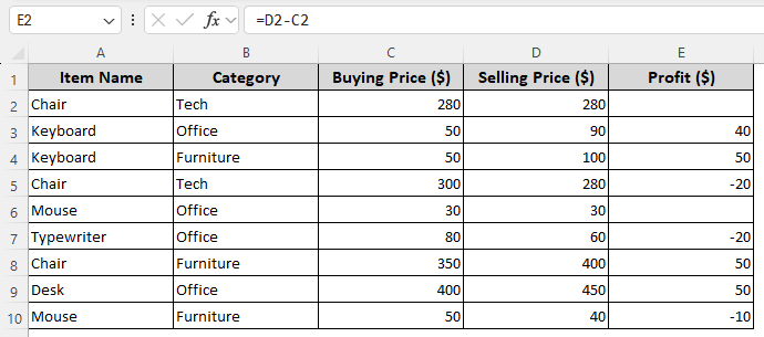
➤ Click Ok and Excel will turn zeros into blanks.
Custom VBA Macro to Set Cells to Blank
To completely clear the content of a cell based on formulas or conditions, you’ll need a VBA macro. Here’s how to customize a macro that converts zeros, negative numbers, errors, and custom conditions into blanks:
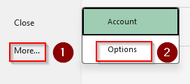
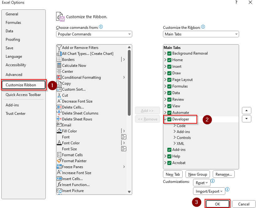
➤ If you can’t find the Developer tab on your main ribbon, go to the File tab >> More >> Options.
➤ Click on Customize Ribbon and check the Developer box in the Main Tabs group. Press Ok.
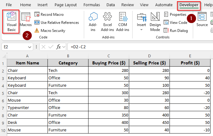
➤ Now, open the Developer tab and choose Visual Basic in the Code group.
➤ As the VBA Editor opens, click on Insert and select Module.

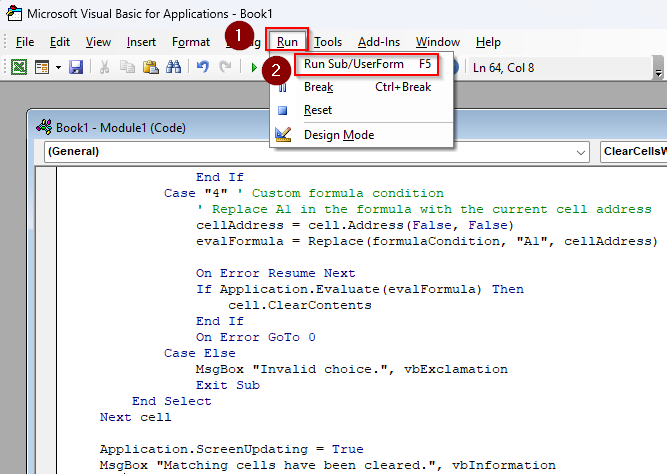
➤ Paste the following code in the blank Module box:
➤ Press the Run button and choose Run Sub/UserForm.
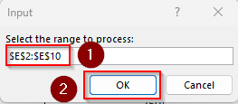
➤ As Excel prompts you to select the range to process, go back to the Excel tab and highlight the cells with the returned values you want to convert. Click
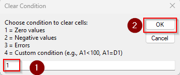
➤ From the Clear Condition box, select a number based on whether you want to set blanks for zeros, errors, or negative values. You can also choose the 4th option to add a custom condition like set blank if A1>100. After entering a number, press Ok.
➤ Here’s the final result for our dataset after setting blanks for zeros:
![]()
Frequently Asked Questions
How to automatically hide all zero values and set blanks?
To hide zeros in the entire sheet, go to the File tab >> More >> Options >> Advanced. Scroll down to find the Display Options for This Worksheet group. Uncheck Show a Zero in Cells That Have Zero Value and click OK.
How to find blank cells in Excel with a formula?
For counting blanks in a range, enter the following formula:
=COUNTBLANK(A1:D10)
Change the range (A1:D10) according to your dataset and press Enter. It counts all empty cells and cells with formulas returning “” in the specified range.
How to fill blank cells automatically?
To automatically fill blanks with a specific value, select your range and press CTRL + G. Click Special and select Blanks from the Go To Special dialog box. In the formula bar, type a value like 0 or N/A and Press CTRL + ENTER to fill all blanks at once.
Concluding Words
All the formulas above return an empty string based on the condition you set. While you can change the formulas, make sure you enter the arguments correctly for the functions to work. Keep in mind that Excel doesn’t identify empty strings as truly blank.
Therefore, functions like COUNTA and ISBLANK don’t count these returned cells. The only way to truly return a blank cell is to use a VBA macro.