
Working in Excel does not often mean working in one worksheet. Due to the complexity and large datasets, we are often required to spread the data into multiple worksheets. However, they often need to be extracted from the other datasets instead of depending on the static references. Thus, the dynamic reference of cells enables you to pull the data from the other sheets based on some conditions and logics. And also transfer it to the existing cells at the end.
To reference cells in another sheet dynamically, you need to follow the steps below:
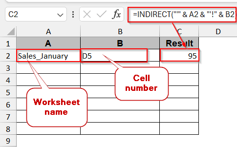
➤ Make a new sheet with three columns for the worksheet name, the cell number of the specific cell, and the resultant value.
➤ In the first column, in the second row (A2), assuming the first row is for headers, write the sheet name.
➤ In the second column, the same row (B2) includes the cell number of the value you want to show.
➤ In the last column of the Result, write the following formula-
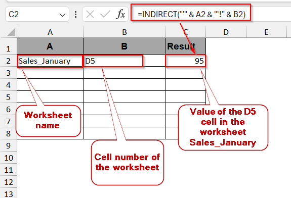
=INDIRECT(“‘” & A2 & “‘!” & B2)
where A2 has a sheet name and B2 contains the cell number of the sheet that needs to be referenced.
➤ Press Enter to dynamically reference the data from another worksheet.
This article will try to make your journey easier when dealing with dynamic references across multiple sheets. We will give a complete step-by-step guide by highlighting the simplest methods like the INDIRECT, CHOOSE, and INDEX functions, the dropdown menu, and even advanced tools like VBA Macros. With interactive examples, workbooks, and frequently asked questions, we will try to cover everything you need.
How Does Dynamic Sheet Referencing Work in Excel?
In simple words, referencing means pulling data from one worksheet to another using formulas and tools. This helps to display the data to the users while dealing with large datasets. This referencing can be of two types – static and dynamic. Static reference only works for the specific sheets and cells.
However, in real life, dynamic referencing is more effective when working with multiple cells and where the target cell might be due to the user selection. It enables the user to create a worksheet based on the target cells and the values present in the other worksheets. This can be easily done by some functions like INSERT and CHOOSE, as well as customized VBA scripts.
The syntax of the formula of dynamic referencing looks like this –
=INDIRECT("'"&A2&"'!"&B2)
where A2 is the separate sheet name and B2 is the target cell whose contents we want to display.
Using the INDIRECT Function to Reference Another Sheet Dynamically
The INDIRECT function is useful for pulling data from different worksheets and displaying it on another worksheet. The best part of this method is that it dynamically updates any data in the new worksheet, even if the original data is changed.
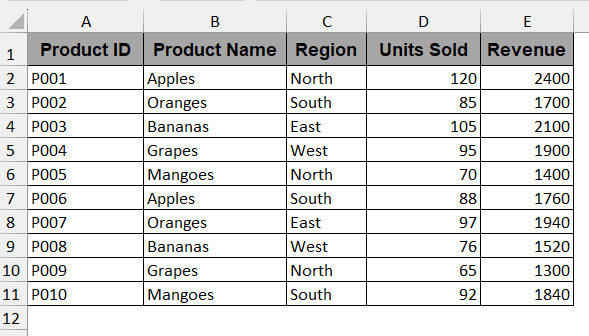
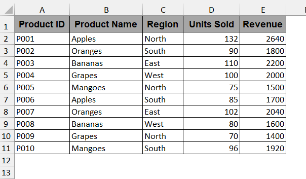
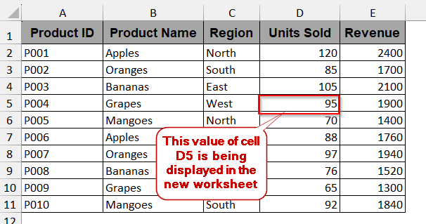
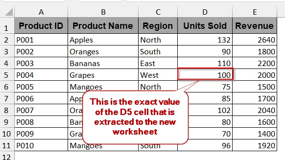
In this example, we have two worksheets, Sales_January and Sales_February, holding the revenue and the sales data of the products. Both worksheets have the same columns and structure, but Unit Sold and Revenue values are different. We want to retrieve the D5 cell value from the Sales_January worksheet to a new worksheet.
Worksheet 1: Sales_January
Worksheet 2: Sales_February
Steps:
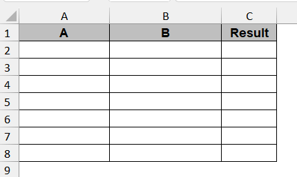
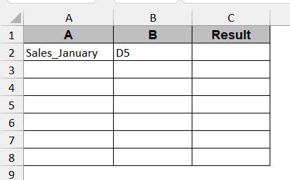
➤ To store the data, make a new worksheet with your preferred name. It will have three columns: one to store the sheet name, another to store the cell number of the sheet name, and the last to hold the resultant value(e.g, A, B, & Result).
➤ In the first row of the first column (excluding the header), for example – A2, write the name of the worksheet in which you want to display the values.
➤ In the second column of the same row (e.g, B2), write the cell number of the cell in the original sheet that holds the required data (e.g, D5).
➤ In the Result column or the third one, write the following formula –
=INDIRECT("'" & A2 & "'!" & B2)
where A2 holds the sheet name and the B2 cell contains the cell number of the specific sheet.
➤ Press Enter to display all the values of that specific cell (D5) in the Result column.
Note:
Make sure to give the apostrophe and use the correct INDIRECT formula to avoid formula breaking.
Referencing Cells Across Sheets via Drop-Down Control
The dropdown control of the sheets can also be used for dynamic referencing. It is simpler when you just want to select the sheet from a menu and extract the data automatically from the sheets. This method itself uses Data Validation tools along with the regular INDIRECT functions to pull the selected data.
Steps:
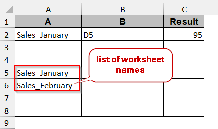
➤ Go to the new worksheet and create three columns just like before. Column A will hold the worksheet name, column B will hold the cell number, and column C will display the extracted value.
➤ Select any of the cells and list the names of the worksheets from which you want to extract the data (e.g., from A5).
➤ List the names vertically, column after column.
➤ Select a cell in column A where you want to display the drop-down list of the worksheets.
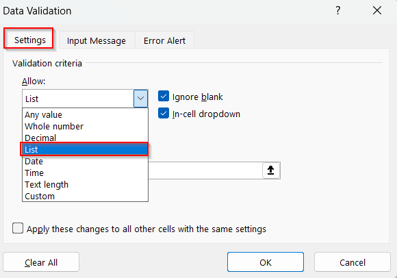
➤ Go to the Data tab -> Data Validation menu in the Data Validation option.
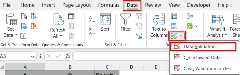
➤ In the Data Validation window, in the Allow option of the Settings tab, choose List.
➤ In the Source, give the cell range where you have listed the worksheet names. And click OK.
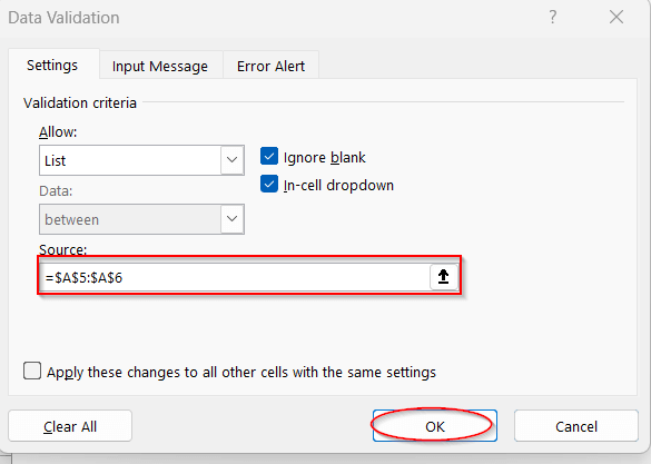
➤ This will create a drop-down menu to choose the worksheet name in the selected cell.
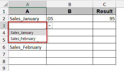
➤ Select the preferred worksheet name, and in the next column of the same row, write the cell number of the data that needs to be referenced.
➤ In the Result column, use the same INDIRECT function –
=INDIRECT("'" & A3 & "'!" & B3)
where A3 contains the worksheet name and B3 contains the cell number of the worksheet.
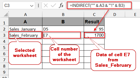
➤ Press Enter to display the data of the referenced cell.
Note:
➨ Write the sheet names exactly as they are, maintaining the casing of the letters. Otherwise, they will not be identified by Excel.
➨ You can always add more sheets in the cell range and add them to the drop-down menu.
Apply Dynamic References with Named Ranges Across Sheets
In Excel, we often need to pull data from specific cell ranges of the sheets regularly. Repeating the same task again and again is time-consuming and not productive. Using the named ranges, you can actually create a label for the specific cell range of the worksheet and reference it. You don’t need to mention the sheet names and the cell numbers time and again.
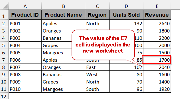
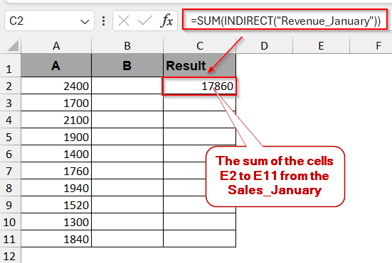
➤ Go to the preferred worksheet and select the range of cells that you need to extract data. For example, we select the range from E2 to E11 for total revenue from the Sales_January worksheet.
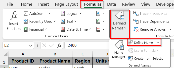
➤ Click on the Formulas tab and select Define Name.
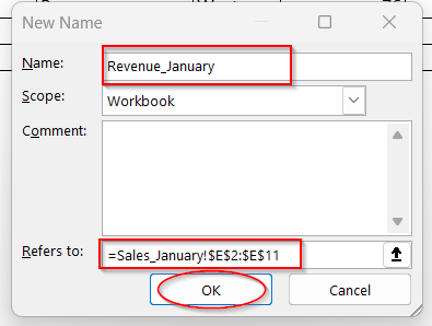
➤ In the window, give your preferred name to the labelled formula. Ensure the Refers to points to the proper cell range before clicking OK.
➤ Repeat the same process for the other worksheets.
➤ After naming is completed, go to your new worksheet.
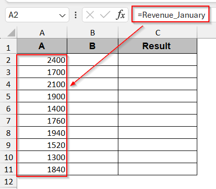
➤ In the preferred cell of the first column, write the formula name. This will extract all the data of the selected range.
➤ In the next column of the same row, use the formula to sum all the values of the selected range of cells-
=SUM(INDIRECT(“Revenue_January”))
where Revenue_January is the label created through the Name Define option.
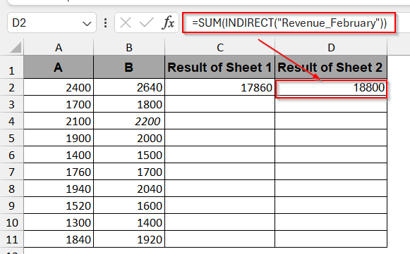
➤ You can also extract and do the same for the other worksheets in the same way.
Note:
➨ Ensure you type the formula in the proper case and with the apostrophe to avoid #REF errors.
➨ You can also use any formula other than SUM based on your requirement.
Automate Dynamic Sheet Referencing with Excel VBA
VBA Macros are your go-to method for reducing manual formula entry. You can easily create customized VBA scripts to extract data from any number of worksheets and cells with a few clicks. This can help you generate dashboards that rely on clicks or events.
➤ Create a new worksheet with the three columns as before.
➤ In the first column (A2) row, excluding headers, write the worksheet name and cell number (B2).
➤ Leave one column beside them for Results.
➤ Go to the Developers tab and click on Visual Basic to launch the VBA editor.
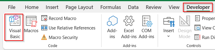
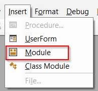
➤ In the window, click on the Insert tab and choose Module to write the VBA script.
➤ Paste the following macro
Sub GetDynamicReference()
    Dim sheetName As String
    Dim cellRef As String
    sheetName = Sheets("VBA Method").Range("A2").Value
    cellRef = Sheets("VBA Method").Range("B2").Value
    On Error GoTo ErrorHandler
    Sheets("VBA Method").Range("C2").Value = Sheets(sheetName).Range(cellRef).Value
    Exit Sub
ErrorHandler:
    MsgBox "Invalid sheet name or cell reference. Please check your inputs.", vbExclamation
End Sub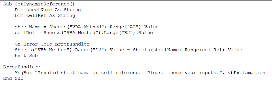
➤ Save the file in the VBA editor and close the window.
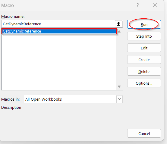
➤ Click on the Macros option in the Developers tab beside the Visual Basic.
➤ From the Macros window, select the name of the formula you just generated and click Run.
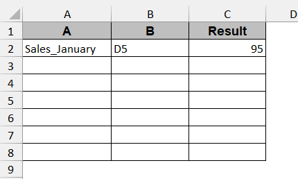
➤ This will generate the cell value of the referenced cell automatically to the first row of column C without any formula.
Note:
After adding the VBA script, save the file as a macro-enabled file to reuse it again.
CHOOSE and INDEX as Alternative to INDIRECT Function
Though dynamic reference is often done with the INDIRECT function, it’s not the best way. The function is volatile. It needs to check and calculate the result every time the worksheet is updated. Additionally, it is not available in many Excel-based platforms either. The best alternative to this is the combination of the CHOOSE and INDEX functions for dynamic referencing.
Steps:
➤ In the new worksheet, make two columns, one for the worksheet name and another for the results. For simplicity, you can also have an intermediate column for tracking the cell numbers, as before.
➤ In the first column, write the worksheet name (e.g, Sales_February).
➤ In the next column of the same row, write the following CHOOSE formula –
=CHOOSE(MATCH(A2, {"Sales_January","Sales_February"}, 0),Sales_January!D5,Sales_February!D5)
Here, Sales_January and Sales_February are the worksheet names, and D5 is the cell number of the required data. Replace this with your sheet name and cell number.
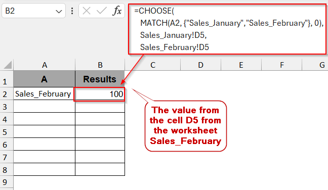
➤ Press Enter to display the extracted value from the original sheet.
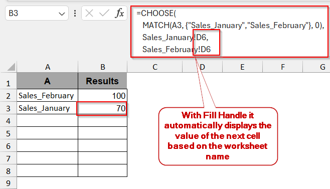
➤ You can also reference the other worksheets by just writing the names in the first column and dragging the cells for the Fill Handle. Though if not modified, the formula automatically displays the value of the next cell number (e.g, D6)
Note:
#NA error can occur if the sheet name in column A does not match the listed sheet name in the formula.
Frequently Asked Questions (FAQs)
Why is my INDIRECT function not working with another sheet?
The INDIRECT function may not work properly on another sheet for several reasons, such as syntax errors or closed workbooks. The workbook that you want to reference must be opened. Along with this, the name, casing, must be properly written with the apostrophes.
Can I use a dynamic sheet reference in a data validation list?
You can use a dynamic sheet reference in a data validation list. Go to the Data tab and select the Data Validation option. However, the data validation option alone will not help; you need an extra INDIRECT function for proper referencing.
How do I update references when a sheet is renamed?
Typically, the formulas and references are automatically updated when your sheet is renamed. Unfortunately, when working with complex functions, VBA methods, or named ranges, you might need to manually update the formulas. Also, you can use the Find and Replace option to adjust these formulas.
How can I dynamically reference a range from another sheet, not just a single cell?
To reference a range of cells, you can use any of the methods, like the INDIRECT function, VBA, or named ranges. It is preferable to use the named range procedure as it is designed to reference a range of cells. You can also modify the INDIRECT formula and use it to extract the ranges –
=SUM(INDIRECT(“‘”&A1&”‘!A1:B10”)),
where A1 to B10 is the selected range
Can I use dynamic sheet referencing in Pivot Tables?
There is no direct formula for dynamic sheet referencing in Pivot Tables. But you can use dynamic referencing using the formula of OFFSET or the named ranges.
How do I prevent #REF errors when referencing sheets dynamically?
The #REF error is common in referencing sheets. To avoid these errors, make sure your cell numbers and the worksheets are properly referenced and spelled. Also, recheck the formulas and their syntax to avoid unwanted errors.
Final Thoughts
Referencing a cell from another worksheet not only makes your data flexible but also reduces the inactivity of some of the worksheets. It is quite helpful for building dashboards, monthly reports, and department summaries. With some of the simplest functions like INDIRECT, CHOOSE, and INDEX, drop-down menus and automated VBA Macros can turn your worksheets into intuitive reports. You can choose any one that fits with your needs and the complexity of the tasks. And, get the clean data structures with the optimal results.