
Commas are frequently used to make large numbers easier to read and comprehend. When you write the numbers like 1000000, Excel may automatically format them as 1,000,000 rather than 1000000. That’s called comma style. But there is a difference in using the comma style in different countries.
Commas are used after every three numbers in the US (1,000,000). However, in India, Nepal, Pakistan, and Sri Lanka, the comma format uses a lakh-crore system, which is equivalent to 10,00,000.
In this article, you will learn how to change the comma styles in Excel using a variety of techniques, including custom choices in positive and negative numbers, Indian-style grouping, and regular US formatting.
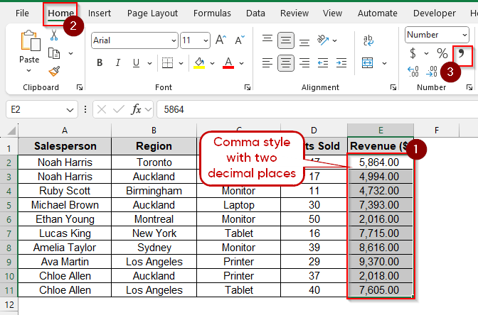
Steps to change comma style to a thousand separator, where 2 decimal places will be shown too:
➤ Select the cells that contain a large number.
➤ Go to the Home tab.
➤ In the Number group, click the Comma Style (,) button, which will display numbers with two decimal places.
This article outlines four different methods for changing comma style in Excel. Changing to Standard US comma Style, converting to Indian style using a custom format, formatting Negative Numbers with US Style Commas and Text Color, and using the Comma Style Button from the Home Tab are the four ways to change the comma style in Excel.
Changing to Standard US Comma Style
In most Western countries, commas are used from right to left after every 3 digits. You can easily display the comma style in the standard US format.
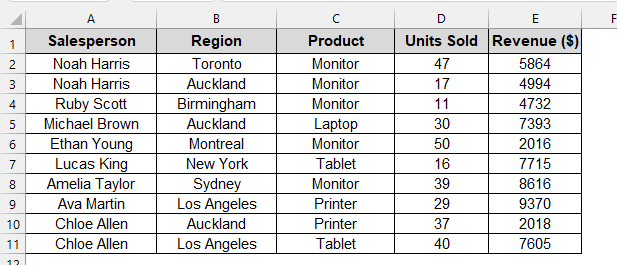
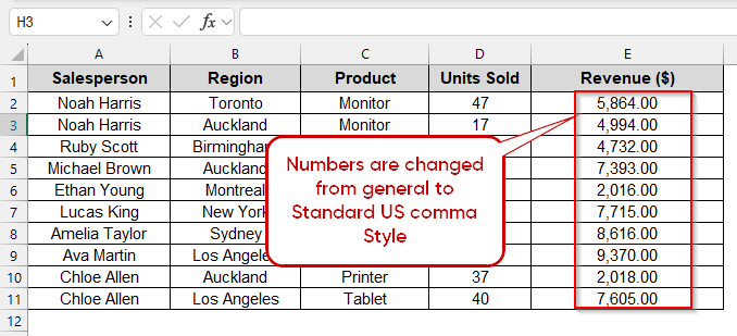
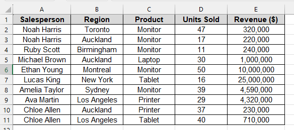
Look at the sales revenue dataset below, where the revenue numbers are generally presented without commas. Now we will change these numbers to standard US comma style.
Steps:
➤ Select the cells E2 to E11
➤ Press Ctrl + 1 to open Format Cells.
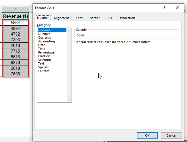
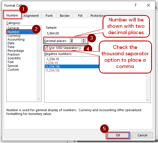
➤ Go to the Number tab.
➤ Choose the Number category.
➤ Check the Use 1000 Separator (,) box.
➤ Set decimal places (2).
➤ Click OK.
➤ Now you can see the output of these steps. General numbers are changed to Standard US Comma Style.
Converting to Indian Style Using Custom Format
In India, Nepal, Pakistan, Sri Lanka, commas are placed after 3 digits from right, then every 2 digits. So a number such as 223344556677 will look like 2,23,34,45,56,677 with the Indian comma style. Now, to show the Indian comma style, you need to set a custom formula.
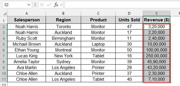
Let’s look at the dataset below, where the column E numbers are shown with Standard US Comma style. We’ll change the values in column E to the Indian comma style format.
Steps:
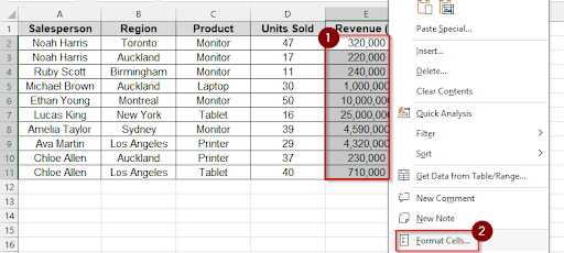
➤ Select the cell range of E2:E11 from column E.
➤ Open the Context Menu with Right-click and select the option Format cells.
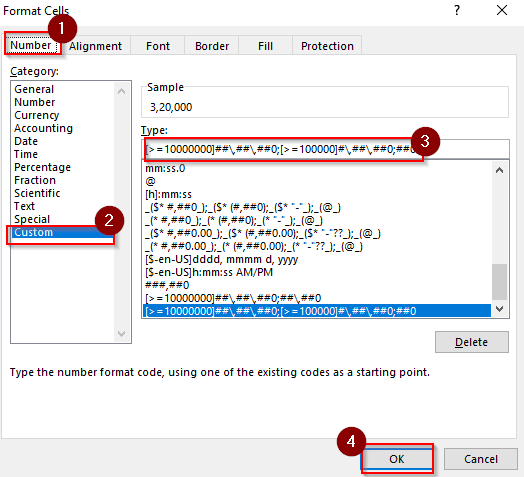
➤ Click Custom (under Number tab).
➤ In the Type field, enter: [>=10000000]##\,##\,##0;[>=100000]#\,##\,##0;##0
➤ Press OK.
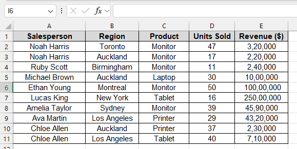
➤ Now you can see the result in column E. The first number was 320,000. After using a custom number format, the number is now 3,20,000. That means the indian comma style is applied from right to left after 3 digits and then 2 digits.
Note:
The formula will work only for numbers greater than 1 lakh.
Format Negative Numbers with US Style Commas and Text Color
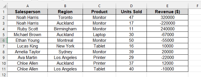
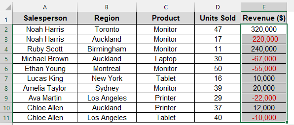
You can show the positive and negative numbers with commas. The comma will be placed after 3 digits from right to left, and you can highlight the negative numbers in red. Let’s look at the dataset below, where the revenue numbers contain some negative numbers.
Steps:
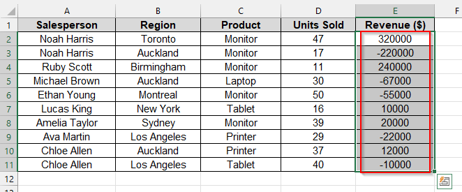
➤ Select the cell range of E2:E11 from column E
➤ Press Ctrl + 1 to open the Format Cells dialog box
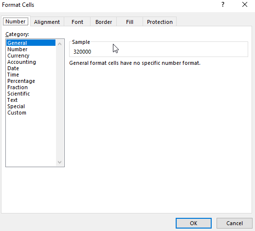
➤ Click the Number tab and go to Custom format.
➤ Use this code: #,##0;[Red]-#,##0
➤ Click OK.
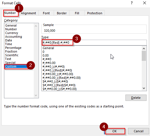
➤ Now you will see the negative numbers are red, and commas are placed after 3 digits from right to left.
Using the Comma Style Button from the Home Tab
There is a built-in comma button in Microsoft Excel which will add a comma in the numbers with decimal places by default. Standard US comma style is the default comma style.
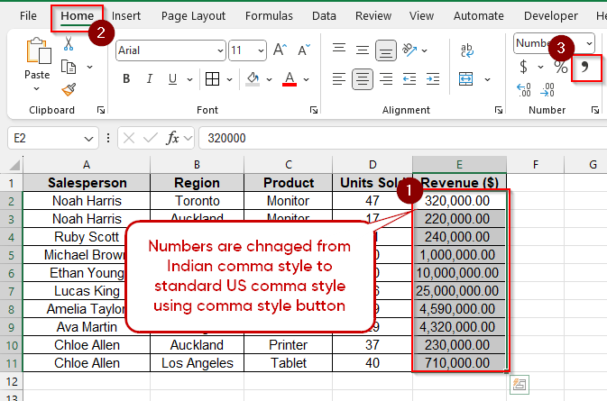
Let’s look at the dataset below, where the column E numbers are shown with Indian comma style. Now we will change the comma style to the standard US comma style by using a comma style button from the Home tab.
➤ Select the cell range of E2:E11 from column E
➤ Go to the Home tab.
➤ In the Number group, click the Comma Style (,) button, which will display numbers with two decimal places.
Frequently Asked Questions
Is there any keyboard shortcut to apply a comma in the numbers?
Yes, using keyboard shortcuts, you can apply the comma style easily. By default, it will display the numbers with 2 decimal places. The keyboard shortcut is: Alt + H + K
Is there any way to remove the decimal places from the numbers after applying the comma style?
Yes, there is a way to remove the decimal places after applying the comma style. In the Format Cells option, click Number, check 1000 separator (, ), and set Decimal Places to 0.
What’s the reason for not showing the comma correctly?
A comma will not show in your Excel file if the cell format is set to text instead of number, if you don’t apply comma style, or if your regional setting and desired format are not matched.
Wrapping Up
In this article, we explored different ways to change the comma style in Excel. We have discussed the standard US style, Indian style and the positive and negative numbers comma style. Feel free to download the practice file and share your thoughts and suggestions.