In Excel, comparing two columns can help you spot differences, check data consistency, or extract meaningful results. This is especially useful when managing lists such as employee attendance, inventory records, or customer orders.
For example, you might have one list of employees who registered for a session and another list of those who actually attended. By comparing the two, you can quickly identify who showed up and who didn’t. Excel offers several formulas that make it easy to perform these comparisons and return helpful results.
In this article, we’ll explore different ways to compare two columns and return a specific value. These methods can be used to flag matches, highlight differences, or pull in related information based on your data.
Here’s how to compare two columns and return a value using the IF function:
➤ Open your dataset in Excel.
➤ Click on cell C2, where you want the comparison result to appear.
➤ Type the following formula:
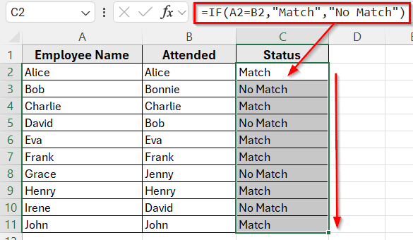
=IF(A2=B2,”Match”,”No Match”)
➤ Press Enter. The formula will compare the values in cells A2 and B2.
➤ If both values are the same, Excel will return Match. If they are different or one is blank, it will return No Match.
➤ Drag the fill handle down to copy the formula for the rest of the rows in Column C.
Use IF Function to Compare Two Columns and Return a Value
In the following dataset, we’re managing a training attendance record. Column A lists all Employee Names, Column B contains names of those who Attended, and Column C will show the result of the comparison.
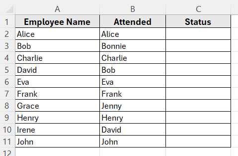
We’ll use this dataset to demonstrate various ways to compare columns and return values in Excel.
One of the simplest ways to compare two columns in Excel is by using the IF function. This method checks if the values in two cells are exactly the same and returns a result based on the comparison.
It is useful when your data is arranged in two parallel columns and you want to quickly see which rows have identical values.
Compare and Return Match or No Match
This method displays clear results such as Match or No Match, which helps you quickly identify identical and different values between columns.
Here’s how to apply this method:
➤ Open your dataset in Excel.
➤ Click on cell C2, where you want the comparison result to appear.
➤ Type the following formula:
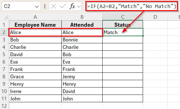
=IF(A2=B2,"Match","No Match")
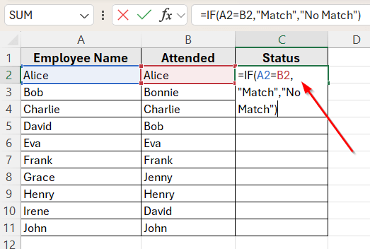
➤ Press Enter. The formula will compare the values in cells A2 and B2.
➤ If both values are the same, Excel will return Match. If they are different or one is blank, it will return No Match.
➤ Drag the fill handle down to copy the formula for the rest of the rows in Column C.

Return Custom Values Based on Match
Instead of showing a generic result like Match or No Match, you might want to display more meaningful terms. For example, in an attendance list, you may prefer using Present or Absent to make the results easier to interpret.
The IF function can be customized to return any text you want based on the comparison result.
Here’s how to apply this method:
➤ Click on cell C2, where you want the result to appear.
➤ Enter the following formula:
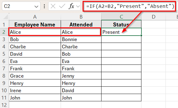
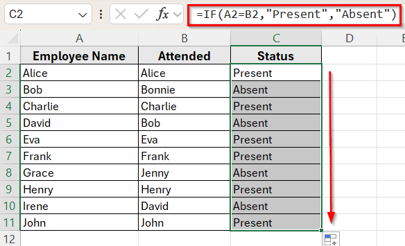
=IF(A2=B2,"Present","Absent")
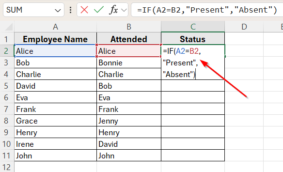
➤ Press Enter. This formula checks if the value in A2 is the same as in B2.
➤ If the two values are equal, Excel will return a Present. Otherwise, it will return Absent.
➤ Drag the fill handle down to apply the formula to the rest of the rows in Column C.
Check If a Value Exists in Another Column Using MATCH Function
Sometimes, you don’t need to compare values row by row. Instead, you may want to check if a value in one column appears anywhere in another column. For example, you might want to see if an employee listed in Column A attended the session, regardless of row order in Column B.
This method uses a combination of the MATCH function and ISNUMBER to search for each value across the entire column.
Here’s how to do it:
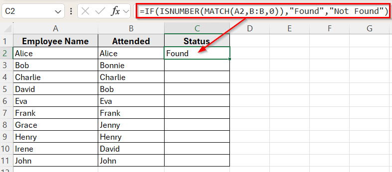
➤ Click on cell C2, where you want the result to appear.
➤ Enter the following formula:
=IF(ISNUMBER(MATCH(A2,B:B,0)),"Found","Not Found")
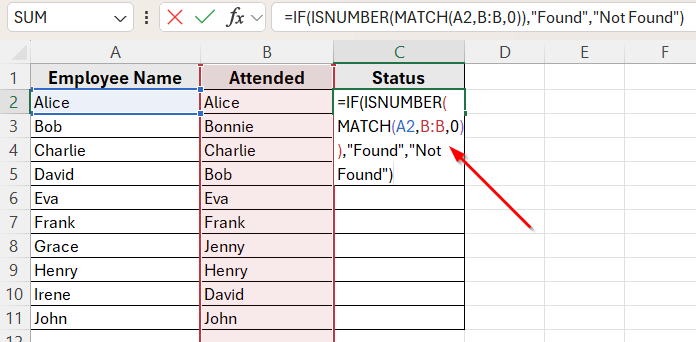
➤ Press Enter. This formula checks if the value in A2 appears anywhere in Column B.
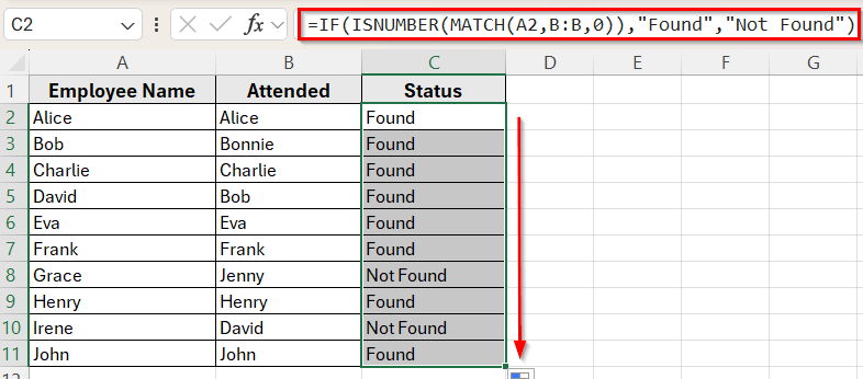
➤ If Excel finds the value in Column B, it returns Found. If not, it returns Not Found.
➤ Drag the fill handle down to apply the formula to the rest of Column C.
Use VLOOKUP to Compare and Return a Related Value
Sometimes, instead of just showing if a match exists, you may want to return additional information related to the match. For example, if an attendee’s name appears in a separate table that also includes their department, you can return the department for each name using the VLOOKUP function.
This method is helpful when you want to pull in data from another table based on a matching value.
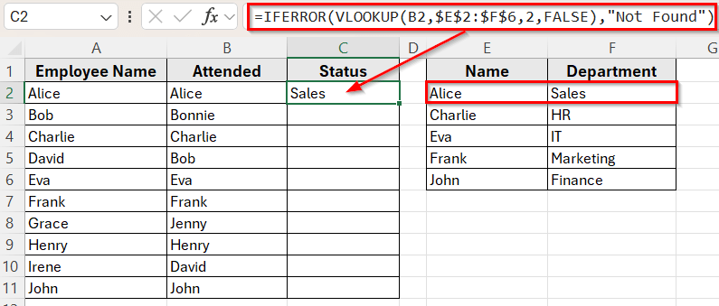
Suppose, you have an extra table in columns E and F that lists employees along with their departments.
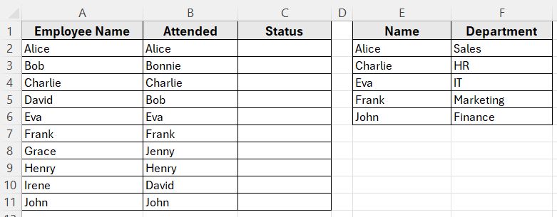
We’ll now look up the department for each name in Column B.
Here’s how to do it:
➤ Click on cell C2, where you want the department name to appear.
➤ Type the following formula:
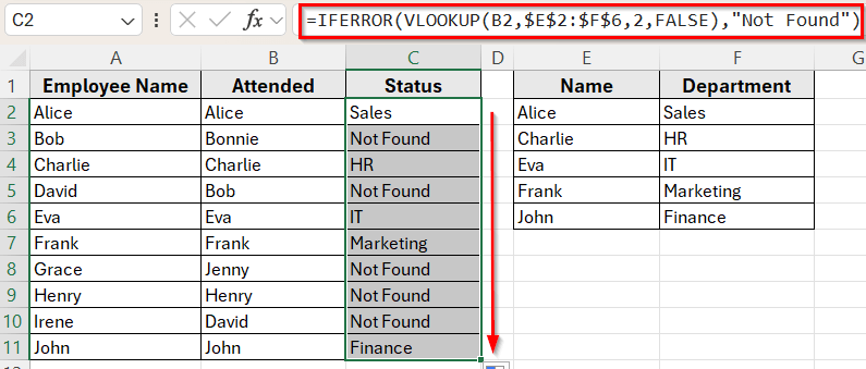
=IFERROR(VLOOKUP(B2,$E$2:$F$6,2,FALSE),"Not Found")
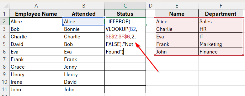
➤ Press Enter. This formula looks for the name in B2 inside the lookup table (E2:F6) and returns the corresponding department from Column F.
➤ If the name is found, Excel returns the department name. If it’s not found, it shows Not Found. In that case, you’ll see the result is Sales which is Alice’s department, according to Column E and F.
➤ Drag the fill handle down to apply the formula to the rest of the rows in Column C.
Highlight Differences Using Conditional Formatting
In some cases, instead of returning a value in a new column, you may want to visually highlight cells that are different between two columns. This helps you quickly scan and identify mismatches without adding extra formulas.
Conditional Formatting is perfect for this. You can apply a color to cells where the values don’t match.
Here’s how to apply this method:
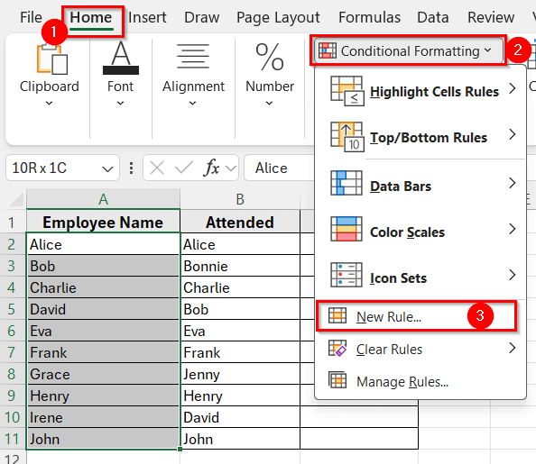
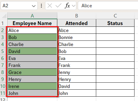
➤ Select the range A2:A11 (the first column you want to compare).
➤ Go to the Home tab on the Excel ribbon.
➤ Click on Conditional Formatting in the Styles group.
➤ Choose New Rule from the dropdown.
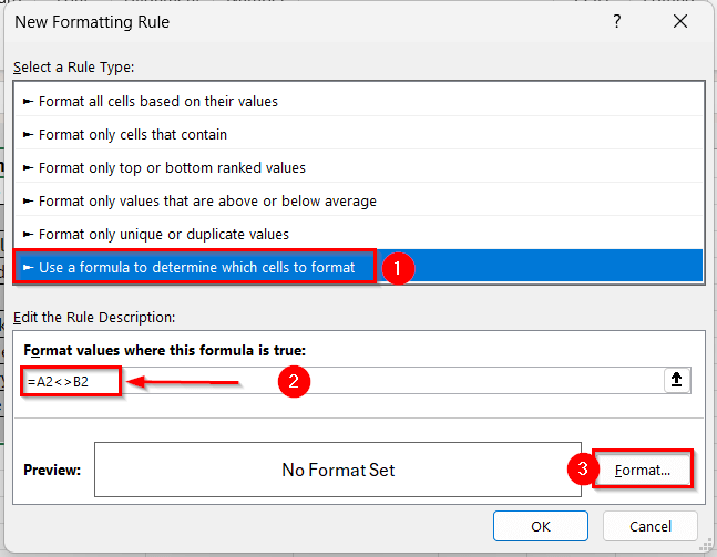
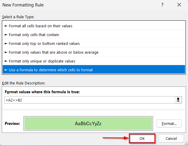
➤ In the New Formatting Rule window, select Use a formula to determine which cells to format.
➤ In the formula box, type
=A2<>B2
➤ Click the Format button.
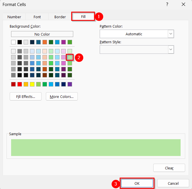
➤ Now, go to the Fill tab, and choose any color you prefer. Then click OK.
➤ Click OK again to apply the rule.
➤ Excel will now highlight any cells in Column A where the value is different from the corresponding cell in Column B.
Note:
You can apply the same rule to Column B by repeating these steps for B2:B11 if you want both sides of the comparison to be highlighted.
Frequently Asked Questions
How do I compare two columns in Excel and return a value?
You can use the IF function like this =IF(A2=B2,”Match”,”No Match”). This checks if the two cells have the same value and returns the result you specify.
How to compare three columns and return a value in Excel?
To compare three columns and return a value only when all three match, you can use a nested IF formula like this:
=IF(AND(A2=B2,B2=C2),”Match”,”No Match”)
This formula checks if the values in cells A2, B2, and C2 are the same. If all three matches, it returns Match; otherwise, it returns No Match. You can customize the return values to fit your context, such as Consistent or Mismatch.
How can I handle errors when a match is not found?
Wrap your formula in IFERROR. For example:
=IFERROR(VLOOKUP(B2,$E$2:$F$6,2,FALSE),”Not Found”) will return Not Found instead of an error message.
Wrapping Up
Excel provides several flexible ways to compare two columns and return a value. You can start with simple IF statements for side-by-side comparisons, or use the MATCH function to look across entire columns. For more advanced tasks, VLOOKUP helps bring in related data. However, Conditional Formatting makes it easy to highlight mismatches visually.
Each method is designed to solve a specific kind of problem, so it’s important to choose the one that works best for your dataset. Try out these formulas in your own Excel file and see how much time you can save when comparing lists.