
Combining text and numbers is often necessary for summaries and labels. For example, for sales data, you might need to integrate the text ‘Total’ with the sales value in numerics to show the total sales amount. When we try to do that directly, using a generic approach, Excel might not be able to do it. It behaves unexpectedly with formatting and formula errors. To avoid these issues, it is best to use your formula or an automated approach.
In order to combine text and numbers in Excel from different cells, go through these steps-
➤ Open the dataset and find the cells that you want to combine.
➤ Create a new column to preserve the result.
➤ Click on the cell, select the first cell, and give an ‘&’ ampersand sign.
➤ In the formula bar, write the text part you want to add or use the TEXT formula to add numeric values.
➤ You can use the direct formula like below –
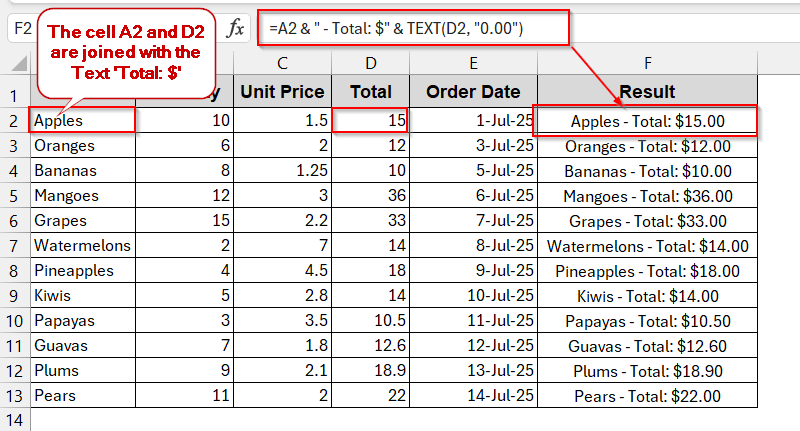
=A2 & ” – Total: $” & TEXT(D2, “0.00”),
where A2 is the first cell, ‘Total: $’ is the text added, and the TEXT formula converts the numeric value of D2 into text to combine them.
➤ Press Enter to get the value in the output cell.
➤ Drag the cells to apply the same formula to the rest of the cells.
Today, we will look into the various methods to combine text and numbers in Excel, including ampersand, CONCAT, and TEXTJOIN formulas. Also, we will discuss the less common ones, like combining them with line breaks and the automated VBA approach. As you walk through all of this, you will not only find the best way for you but also identify common errors and issues, and where exactly you went wrong.
Use Ampersand (&) To Combine Text And Number
The Ampersand operator is the most basic and beginner-friendly approach that you can try. It lets you join different cells, whether adjacent or not, and make them readable. Combining them with some formatting, like the TEXT formula, can make the method error-free even if you have numbers with decimal values.
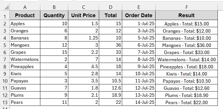
The following dataset will be used to describe all these methods.
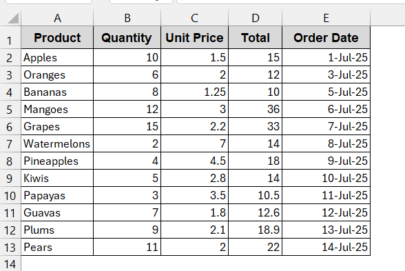
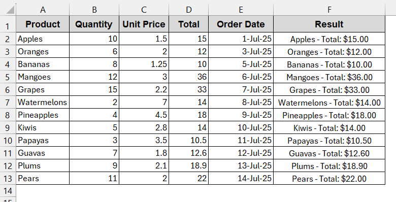
In this method, we will combine the product name and the total with the text ‘Total: $’ to display the total price of each product.
Steps:
➤ Locate the cell numbers or the columns that you want to combine.
➤ Create a separate column to store the combined result with an appropriate header.
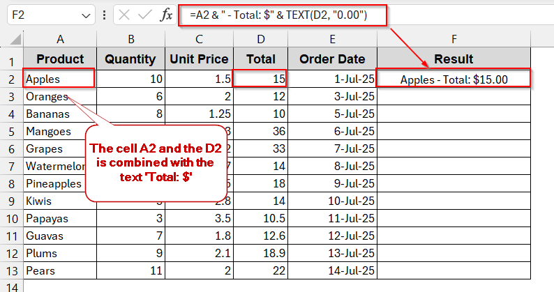
➤ Click the first cell of the new column and write the formula –
=A2 & " - Total: $" & TEXT(D2, "0.00")
where A2 is the first cell of the Product column and D2 is the first cell of the Total column. The text of ‘Total: $’ is added with the ampersand(&) here.
➤ Press Enter to generate the combined result in the output cell.
➤ Drag the cells or use Fill Handle to apply the same formula for the rest of the cells in the column.
Note:
➨ The TEXT function is used to resolve the formatting issue of the numeric value of the column Total. Without wrapping with this formula, the decimal values are displayed correctly.
Join Text and Numeric Values with CONCAT Function
A cleaner version of the first method is using the CONCAT function. It is best when you need to combine long texts or multiple fields. Without relying on the ampersand, this method can help you join texts, numbers, and also cell references.
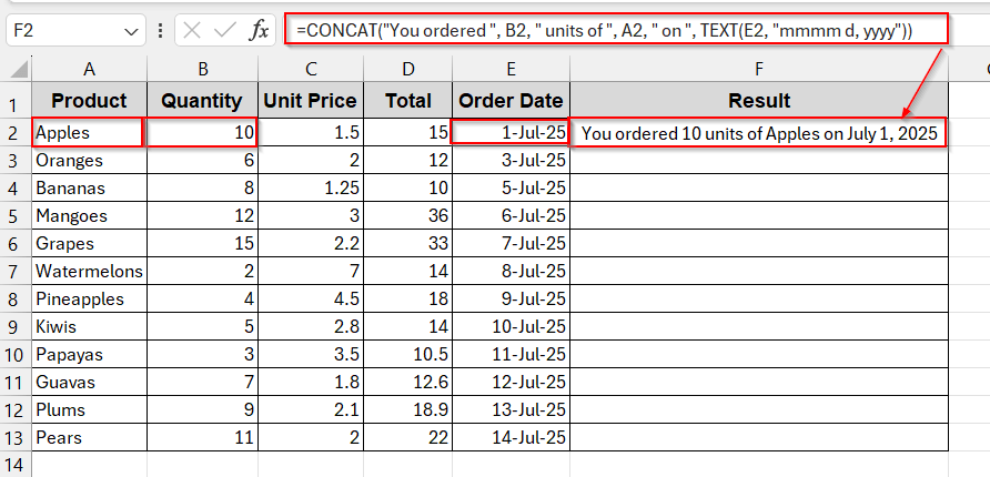
Here, we will add three cell values with external texts. – Quantity, Product, and Order Date.
Steps:
➤ Choose the cell numbers or columns that you want to combine (e.g, A2, B2, E2).
➤ Create a column for storing the result with a proper heading (e.g., Result).
➤ Click and write the formula below –
=CONCAT("You ordered ", B2, " units of ", A2, " on ", TEXT(E2, "mmmm d, yyyy"))
where B2, A2, and E2 are the first cell of the Quantity, Product, and Order Date, respectively. The texts ‘You ordered’, ‘units of’, and ‘on’ are added to the numeric values.
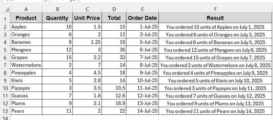
➤ Press Enter to get the result in the cell.
➤ Drag the cells or use the Fill Handle to generate the same formula for the rest of the cells.
Notes:
➨ For older versions of Excel, use the CONCATENATE function instead of CONCAT.
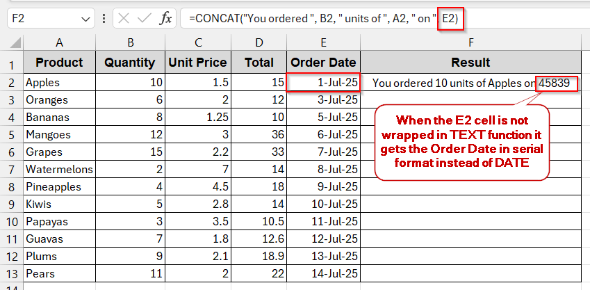
➨ The TEXT function wraps the Order Date to get the output in DATE instead of serial format.
Make Multi-Line Labels by Merging Text and Numbers
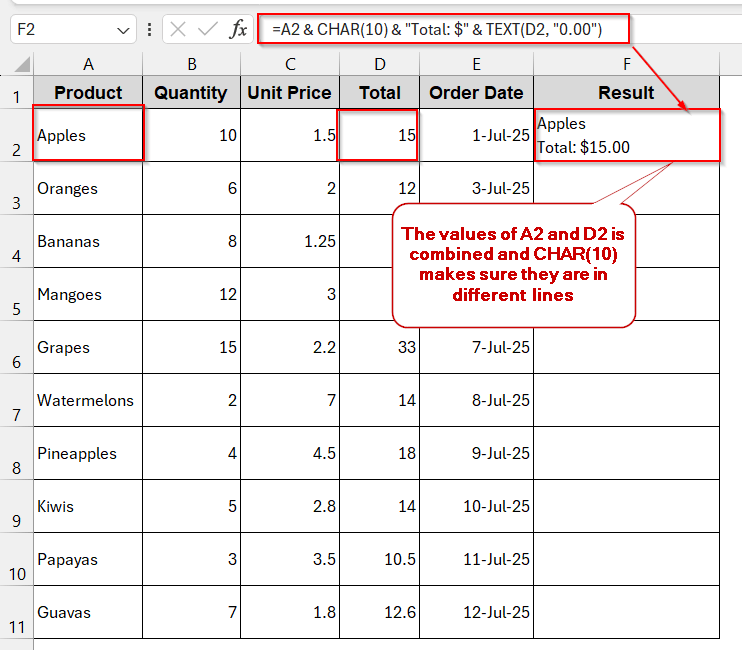
As you have experience, combining long texts and multiple lines can make the cell larger and not readable. Sometimes, writing them in the next line by giving a line break looks better. To do this, we can use the CHAR(10) function to make stackable and interactive labels.
In this method, we will combine the product name and the total value with text.
Steps:
➤ Find the cells that you want to combine in multi-line format. Here, it is A2 and D2.
➤ Make a result column to store the results of the output.
➤ On the output cell, write the following formula –
=A2 & CHAR(10) & "Total: $" & TEXT(D2, "0.00")
where A2 and D2 are the first cells of the Product and Total, respectively.
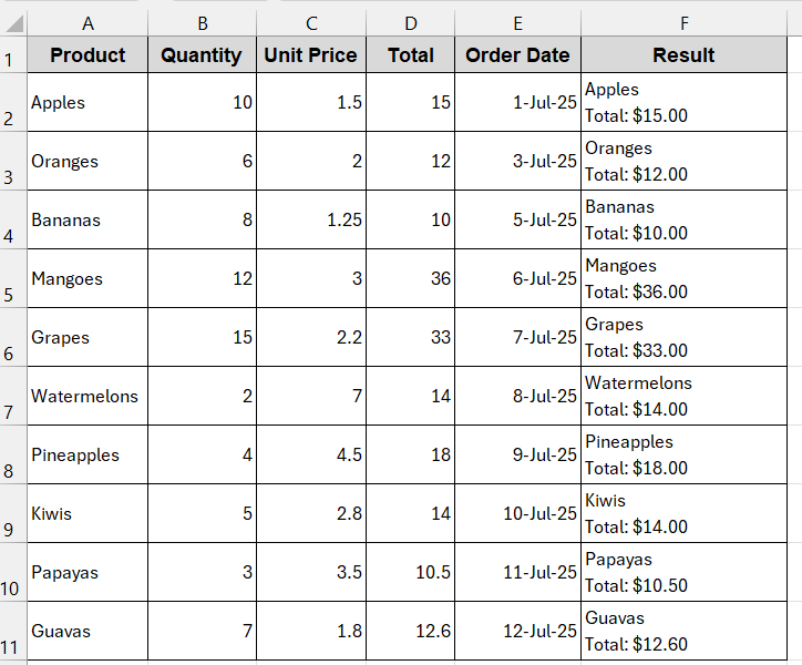
➤ Press Enter to get the combined output in multiple lines.
➤ Use Fill Handle or drag the cells to formulate the rest of the cells in the same formula.
Notes:
➨ CHAR(10) only works for Windows. For MAC, you will need to use CHAR(13) or both CHAR(10) and CHAR(13).
➨ Ensure your cells have Wrap Text enabled to get the result in multiple lines.
Combine Texts and Numbers with TEXTJOIN for Cleaner Formatting
When adding too much data or information in one cell, the general formula of ampersand and CONCAT seems messy. Though you can obviously get the desired result with them, people prefer to use a cleaner and smarter approach like TEXTJOIN. It helps you join multiple cell values and texts, use a custom delimiter, and even skip blanks. All in one.
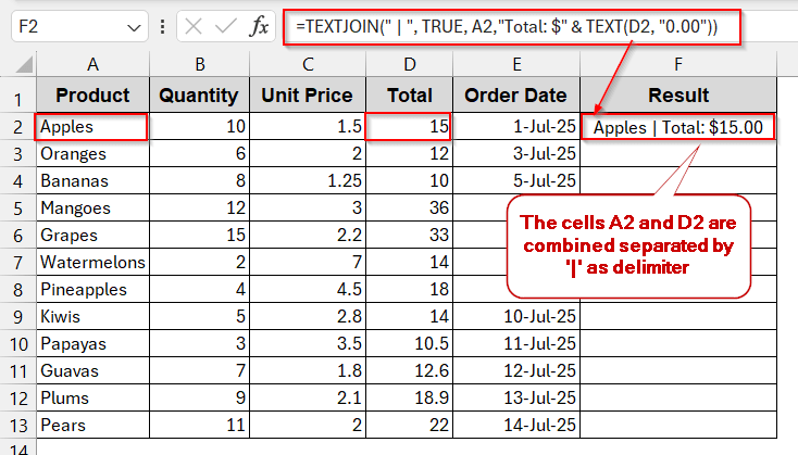
Like the previous one, in this method, we will combine the Product and the Total price. But we will use a delimiter ‘|’ to separate the two cell values.
Steps:
➤ Find the cells you need to combine (e.g, A2 and D2).
➤ Create a custom column with a proper header (e.g, Results) to store the combined result.
➤ Use the below TEXTJOIN formula –
=TEXTJOIN(" | ", TRUE, A2, "Total: $" & TEXT(D2, "0.00"))
where A2 and D2 are the cell numbers of Products and Total respectively.
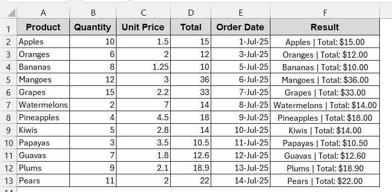
➤ Press Enter to get the output in the Result column.
➤ Drag the cells to apply the same formula to the rest of the cells.
Notes:
➨ TEXTJOIN is not available for versions of Excel older than 2016.
➨ You can use any delimiter, including a comma, a semicolon, and even the CHAR(10) for multi-line.
➨ The parameter TRUE inside the TEXTJOIN function resolves the double delimiter if there is any blank space. You can also use ignore_empty instead of TEXTJOIN.
VBA Macro to Combine Texts and Numbers with Formatting
If you’re working with large datasets and don’t have the time and energy to copy or manually write the formulas, you can go for VBA Macros. It’s custom-made and formulated once, and you can use it for a lifetime. Plus, it saves you the hassle of formatting, keeping your data cleaner.
Steps:
➤ First, create a new column to store the combined data results.
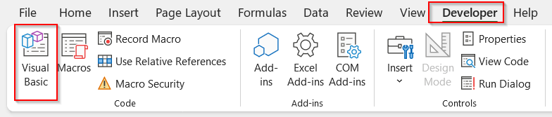
➤ Go to Developers tab -> Visual Basic.
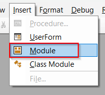
➤ This will launch the VBA editor window. Click on the Insert tab -> Module.
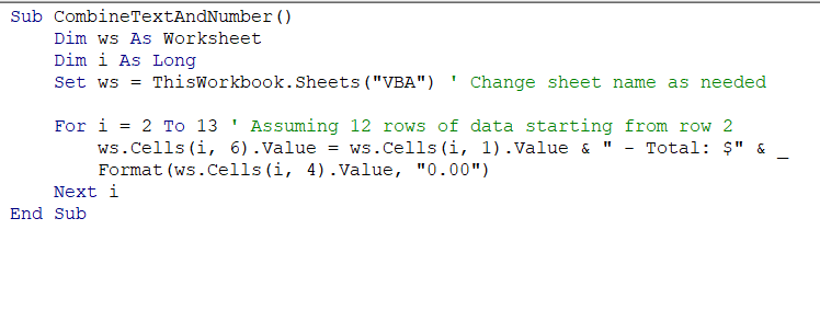
➤ Paste the following VBA code in the blank space-
Sub CombineTextAndNumber()
    Dim ws As Worksheet
    Dim i As Long
    Set ws = ThisWorkbook.Sheets("VBA") ' Change sheet name as needed
    For i = 2 To 13 ' Assuming 12 rows of data starting from row 2
        ws.Cells(i, 6).Value = ws.Cells(i, 1).Value & " - Total: $" & _
        Format(ws.Cells(i, 4).Value, "0.00")
    Next i
End Sub
➤ Save the VBA script by Ctrl + S into a macro-enabled workbook.
➤ Now, again, go to the Developer tab and select Macros beside Visual Basic.
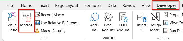
➤ In the Macros window, the name of the custom formula created by VBA will be listed here: CombineTextAndNumber. It is usually the first line of the VBA script after Sub.
➤ Select the custom formula and click on Run.
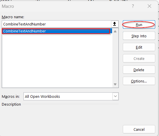
➤ This will automatically generate the entire column with the combined result.
Notes:
➨ Change line 4 with your sheet name in the place of ‘VBA’.
Set ws = ThisWorkbook.Sheets(“VBA”)
➨ Change the column references from lines 6 and 7.
ws.Cells(i, 6).Value = ws.Cells(i, 1).Value & ” – Total: $” & _
Format(ws.Cells(i, 4).Value, “0.00”)
Here, Cells(i,6) refers to column F, which is the output column, Cells(i,1) is Column A (Product), and Cells(i,4) is Column D (Total).
Combine Text and Number with Excel Power Query
If you do not want either formulas or complex VBA scripting, there is still a great way for you. Power Query is not much simpler, but it is also cleaner and more structured in combining texts and numbers. It allows and works with the transformation outside the grid, giving you better formatting capabilities.
In this method, we will combine the text of the Product with the numeric value of Total.
Steps:
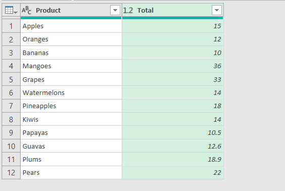
➤ Open your dataset and confirm which columns you want to combine.
➤ Select the ranges of the columns that you want to combine (e.g, A1–A13 and D1 to D13)
➤ Confirm the dialog box with the proper ranges and check the box My table has headers. This will launch the Power Query Editor Window.
➤ Go to the Add Column tab and click on Custom Column.
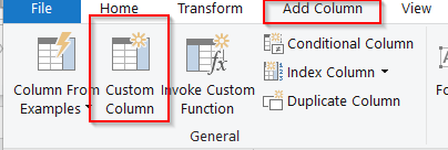
➤ In the Custom Column window, replace the new column name as you require and write the formula below in the Custom column formula box-
=[Product] & " - Total: $" & Number.ToText([Total], "0.00")
where Product and the Total are names of the columns and Number.To.Text formula ensures proper numeric formatting.
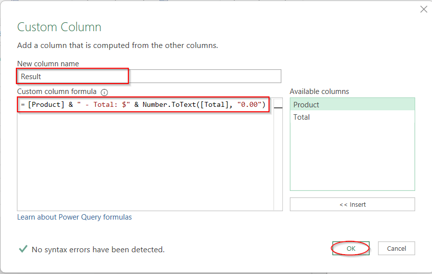
➤ Click OK to create a new column with the combined result in the Power Query Editor.
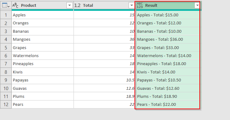
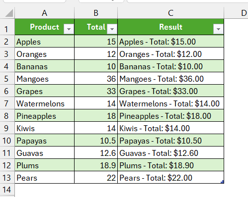
➤ Now, click on the File tab -> Close and Load to load this sheet into a new sheet in your Excel workbook.
Notes:
➨ Does not affect your original worksheet. To load into the original worksheet, choose the Close and Load To option under Close and Load.
➨ You can add data to the table and refresh it to get the combined result for the new rows.
Frequently Asked Questions (FAQs)
How can I combine text with a percentage in Excel?
To combine the text with a percentage in Excel, you can use any of the methods, like Ampersand, CONCAT, or TEXTJOIN. However, to preserve the percentage formatting, wrap the percentage value with the TEXT function. Use the following syntax-
TEXT(B2, “0%”),
where B2 is the cell containing a percentage value.
Why does my combined text lose the currency symbol?
Your combined text might lose the currency symbol due to the formatting issues. To resolve them, use the TEXT function to write the cell reference of that cell.
TEXT(A2, “$0.00”).
Is there a way to combine text and numbers without formulas?
You can combine text and numbers without formulas by using an automated VBA approach. It helps you create a VBA code snippet from scratch, which you can use repeatedly.
Is it possible to combine text and numbers from non-adjacent cells dynamically?
The non-adjacent cells containing text and numbers can also be combined. Any methods, including the ampersand, CONCAT, and even VBA, can join the cell values dynamically, irrespective of their adjacency.
Can I use Power Query to combine text and numbers in a structured way?
Power Query can also combine text and numbers in a structured way. By opening the Power Query window, go to Add Column -> Custom Column. There you will find the join fields option with the formatting benefits.
Concluding Words
We know how frustrating it is to combine text and numbers in Excel. But we can assure you, it can be a lot easier if you know the quick hacks. Using the simple formulas with formatting TEXT functions, tweaking automated VBA, or working hands-on with Power Query – you can always get the best one that matches your layout. Without stressing out, download our workbook and try all of it yourself. Hopefully, joining text and numbers will no longer seem to be a problem.