In HR, payroll, and employee records, you often need to calculate employee tenure based on their joining date and today’s date. Tenure tells you how long someone has worked, expressed in years and months.
Manually calculating tenure can be time-consuming, especially with large datasets. However, Excel provides formulas that make this process simple and accurate. You can use built-in functions like DATEDIF, YEARFRAC, INT, ROUND, DAYS, and LET to calculate tenure in different formats.
In this guide, you will learn simple methods to calculate tenure in Excel in years, months, and a combined format.
Here’s how to calculate tenure in years and months in Excel using DATEIF function:
➤ Open your dataset in Excel.
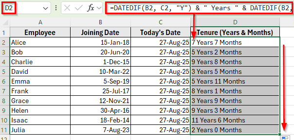
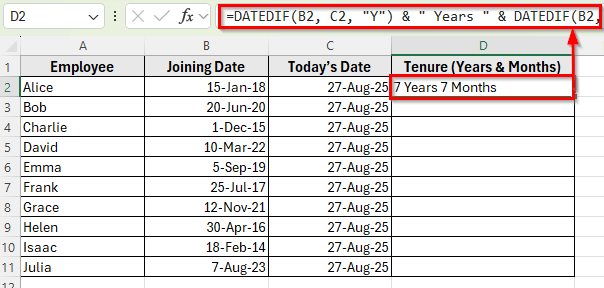
➤ Click on cell D2 and enter the following formula:
=DATEDIF(B2, C2, “Y”) & ” Years ” & DATEDIF(B2, C2, “YM”) & ” Months”
➤ Press Enter. Excel will return the tenure in the format X Years Y Months for cell A2. For example: 7 Years 7 Months.
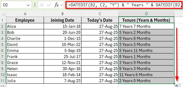
➤ Drag the fill handle down from the rest of the rows to copy the formula for the other employees.
Using DATEIF Function to Calculate Tenure in Years and Months
In the following dataset, we have an employee record with joining dates. Column A lists the Employee Names, Column B contains their Joining Dates, and Column C shows Today’s Date. Column D is empty, where we’ll enter formulas to calculate tenure.
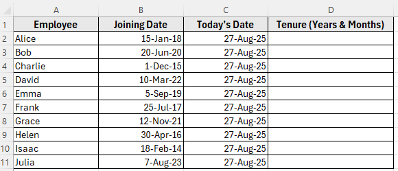
We’ll use this dataset to calculate the tenure in years and months using different formulas.
The DATEDIF function is the most common way to calculate tenure in Excel. It measures the difference between two dates and can return results in years, months, or days. In this method, we’ll use it to find the number of completed years and months of service for each employee based on their joining date and today.
Here’s how to apply this method:
➤ Open your dataset in Excel.
➤ Click on cell D2 and enter the following formula:
=DATEDIF(B2, C2, "Y") & " Years " & DATEDIF(B2, C2, "YM") & " Months"
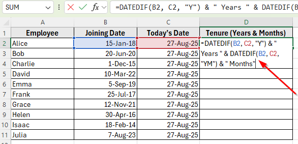
➤ Press Enter. Excel will return the tenure in the format X Years Y Months for cell A2. For example: 7 Years 7 Months.
➤ Drag the fill handle down from the rest of the rows to copy the formula for the other employees.
Combining INT and ROUND Functions to Calculate Tenure
Another way to calculate tenure is by using the functions like INT and ROUND. This method is useful when you want tenure broken into years and months.
Here’s how to apply this method:
➤ Open your dataset in Excel.
➤ Click on cell D2 and enter the following formula:
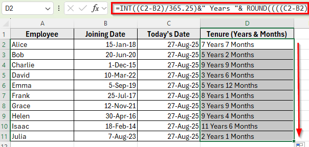
=INT((C2-B2)/365.25)&" Years "& ROUND((((C2-B2)/365.25)- INT((C2-B2)/365.25))*12,0)&" Months"
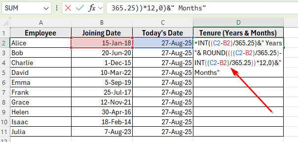
➤ Press Enter. Excel will return Alice’s tenure in years and months in the format X Years Y Months. For example: 7 Years 7 Months.

➤ Drag the fill handle down from cell D2 to D11 to copy the formula for the rest of the employees.
Note:
This method provides an approximate result since it divides total days by 365.25. This approximation assumes every year is 365.25 days, but in reality, the exact number of days between two dates depends on the calendar months.
Use the DAYS Function to Calculate Tenure in Years and Months
This method calculates tenure by first determining the total number of days an employee has worked using the DAYS function. You then convert the days into years and months using a formula.
Here’s how to apply this method:
➤ Open your dataset in Excel.
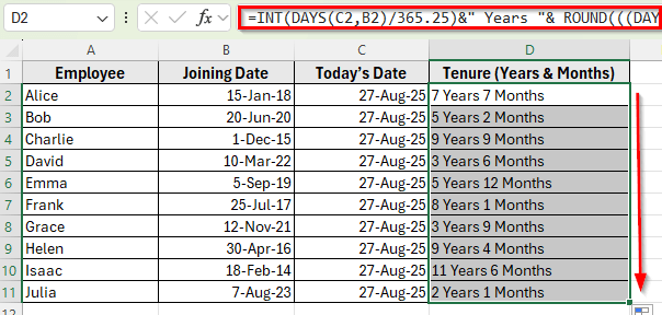
➤ Click on cell D2 and enter the following formula:
=INT(DAYS(C2,B2)/365.25)&" Years "& ROUND(((DAYS(C2,B2)/365.25)- INT(DAYS(C2,B2)/365.25))*12,0)&" Months"
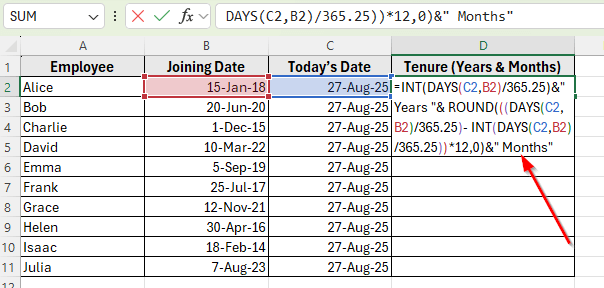
➤ Press Enter. Excel will return Alice’s tenure in the format X Years Y Months. For example: 7 Years 7 Months.

➤ Drag the fill handle down column D to copy the formula for the rest of the employees.
Note:
This method also gives an approximate result like the previous method since it divides total days by 365.25. However, it is useful for estimates and calculations, but small differences can occur in some cases.
Applying the LET Function to Simplify Tenure Calculation
If you are using Excel 365, you can apply the LET function to calculate tenure in years and months in a cleaner way. LET function allows you to define variables inside a formula, so you do not have to repeat the same calculation multiple times.
Here’s how to apply this method:
➤ Open your dataset in Excel.
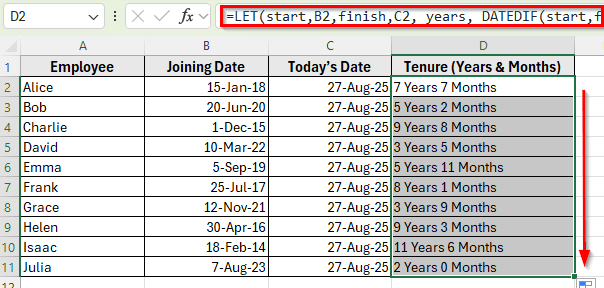
➤ Click on cell D2 and enter the following formula:
=LET(start,B2,finish,C2, years, DATEDIF(start,finish,"Y"), months, DATEDIF(start,finish,"YM"), years & " Years " & months & " Months")
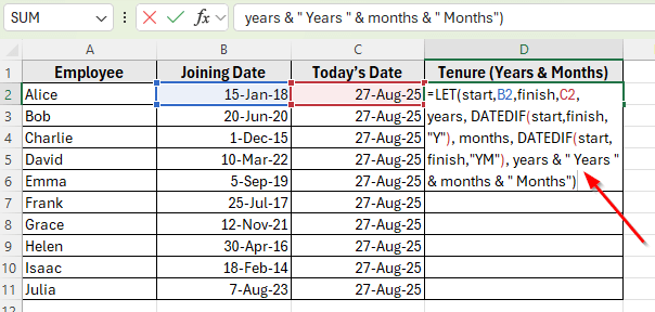
➤ Press Enter. Excel will return Alice’s tenure in the format X Years Y Months. For example: 7 Years 7 Months.
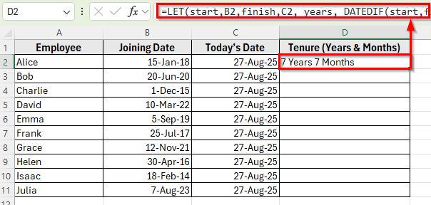
➤ Drag the fill handle down from cell D2 to D11 to copy the formula for the rest of the employees.
Frequently Asked Questions
How to calculate duration in years and months in Excel?
You can calculate tenure by using functions like DATEDIF, DAYS, INT, ROUND, or LET. DATEDIF is the most common method to get completed years and months between the Joining Date and Today’s Date.
How to calculate tenure in years?
You can use the DATEIF function to calculate tenure in years. Here’s the formula:
=DATEDIF(B2, C2, “Y”)
This formula returns the tenure based on the value of cell B2 and C2.
Can I use these formulas in older versions of Excel?
Yes. Most formulas like DATEDIF, INT, ROUND, and DAYS work in almost all Excel versions. The LET function is available only in Excel 365.
Wrapping Up
Calculating tenure in Excel helps you simply see how long employees have worked and makes HR reports easier to read. You can display tenure in years, months, or both together, which keeps your data clear and professional.
Each method suits different needs. DATEDIF gives exact calendar years and months, INT and ROUND or DAYS work with total days, and LET keeps formulas simple in Excel 365.
Using these formulas saves time, avoids manual errors, and helps keep employee records accurate and up-to-date.