
Common lookup functions like VLOOKUP or MATCH usually return a single result for a given lookup value. However, sometimes we need to find all the matched values from a selected range based on a single parameter. Although there’s no single function to achieve this, you can combine several functions to get multiple values in a single cell or as an array.
Combining the TEXTJOIN and IF functions allows you to return all the matched values in a single cell separated by a defined delimiter.
Steps to return multiple values based on single criteria with the TEXTJOIN and IF functions:
➤ Enter the criteria in a blank cell (F2) and enter the following formula in a different cell(G2):
=TEXTJOIN(“, “, TRUE, IF(B1:B10=F2, C1:C10, “”))
➤ Here, B1:B10 is the criteria range and C1:C10 is our return/lookup range. If any cell of column A meets the criteria in F2, this cell returns all the corresponding values from column B, separated by a comma (,).
➤ Change the ranges as needed and press Enter in Excel 365/2021 versions. For older versions (2019 or prior), click CTRL + SHIFT + ENTER .

Depending on how you want the returned output, you can combine other functions like FILTER, INDEX, MATCH, ROW, SMALL, etc. This article covers all the ways of returning multiple outputs based on a single criteria using functions, Power Query tool, and VBA coding.
Returning Multiple Values Based on a Condition Using FILTER Function
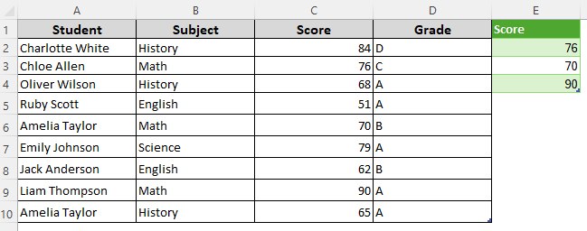
To visually demonstrate the methods, we’ll use a student marksheet dataset with columns for student name, subject, and obtained marks. Our goal is to find the value Math from column B and return the corresponding marks for a match in column C.
So, we entered the value Math in cell F2 to use it as a reference in the formulas. We’ll insert the formulas in cell G2 to list the returned matches.
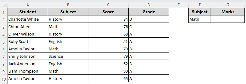
In Excel 365/2021, the FILTER function returns an array of data from a range based on specified criteria. To use this, follow the steps given below:
➤ Select a blank cell to input the returned values and enter any of the the following formulas:
To Match A Cell Reference to A Single Column
➤ Type the criteria you’re matching in a blank cell (F2) and enter the following formula in a different output cell (G2):
=FILTER(C1:C10, B1:B10=F2)
➤ Press Enter to return an array of matched values.
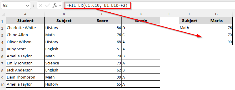
To Match A Value to A Single Column
Select an output cell and enter the following formula:
=FILTER(C1:C10, B1:B10=”Math”)
➤ Click Enter.
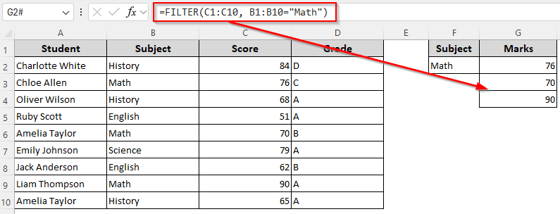
To Match Across Multiple Columns
=FILTER(C1:D10, B1:B10=F2)
➤ In cell F2, we put the criteria or value we’re looking for. B1:B10 is our criteria range where we’re looking for the value. As C1:C10 is our return range or lookup array, Excel will return multiple values from this range corresponding to the matched cells in column B. Replace them based on your dataset.
➤ Press Enter and Excel will return all the matches across rows and columns.
Returning an Array of Matched Results
If you’re using an older version (Excel 2019 or prior), you need to combine multiple functions to get multiple results for a match. A combination of IF and ROW functions compares values in a specified range and returns the row numbers.
While the SMALL function separates the smallest row number, the INDEX function retrieves the value from the lookup range for that position. Finally, IFERROR function returns a blank instead of error if no match is found. Below are the steps:
➤ In a blank cell for the returned value, insert any of the following formulas:
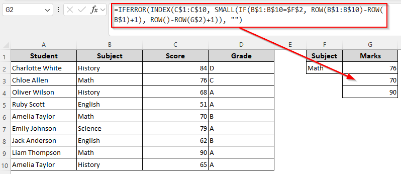
Enter the Results in a Column
To drag the formula down to multiple column cells, enter this formula in the output cell:
=IFERROR(INDEX(C$1:C$10, SMALL(IF(B$1:B$10=$F$2, ROW(B$1:B$10)-ROW(B$1)+1), ROW()-ROW(G$2)+1)), “”)
➤ Change the lookup array C$1:C$10, criteria B$1:B$10=$F$2, and output cell reference G$2 according to your dataset.
➤ For new Excel versions (Excel 365/2021), press Enter to insert the formula. If you’re using an older version (Excel 2019/prior) press CTRL + SHIFT + ENTER . Drag the formula down until Excel returns blank strings.
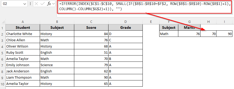
Enter the Results in a Row
To drag the formula across the columns in a row, insert this formula in the output cell:
=IFERROR(INDEX($C$1:$C$10, SMALL(IF($B$1:$B$10=$F$2, ROW($B$1:$B$10)-ROW($B$1)+1), COLUMN()-COLUMN($G$2)+1)), “”)
➤ Replace the lookup array $C$1:$C$10, criteria $B$1:$B$10=$F$2, and output cell reference $G$2 according to your dataset.
➤ Press Enter or CTRL + SHIFT + ENTER depending on your Excel version. Drag the formula across using the fill handle (+ sign on the bottom of the corner).
Using the TEXTJOIN and IF/FILTER Functions Return Multiple Values in a Cell
Both IF and FILTER functions look for matches based on the given criteria. The TEXTJOIN function joins the returned values with a defined delimiter like a comma (,). Let’s learn how to use them:
➤ Enter any of the following formulas in a blank cell for returned values:
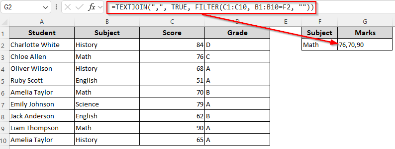
For All Excel Versions
➤ Insert this formula in the output cell:
=TEXTJOIN(“, “, TRUE, IF(B1:B10=F2, C1:C10, “”))
➤ Press ENTER for new Excel versions and CTRL + SHIFT + ENTER for the older ones.

For New Excel Versions
➤ In the output cell, type this formula:
=TEXTJOIN(“,”, TRUE, FILTER(C1:C10, B1:B10=F2, “”))
➤ Click Enter.
Finding Multiple Values Based on Single Criteria with the Power Query Tool
If you want to get multiple values matching the criteria without a formula, using the Power Query tool is a great dynamic solution. For this, follow the steps given below:
➤ Select your data range and right-click on it to get the mini toolbar. Choose Get Data From Table/Range from the options.
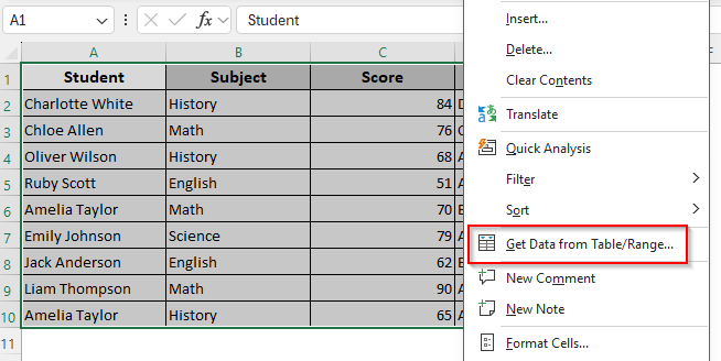
➤ If Excel prompts you to turn the range into a table, press Ok.
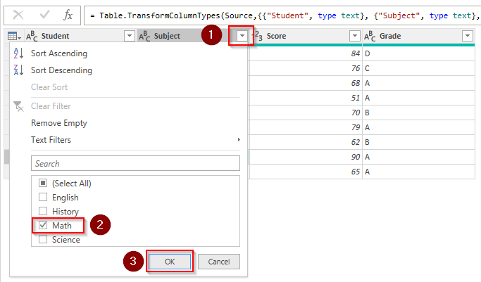
➤ In the Power Query Editor, click the filter drop-down on the column containing the criteria range or value you’re matching. Now, select the value to match and press Ok. Excel will only display rows where the value is found.
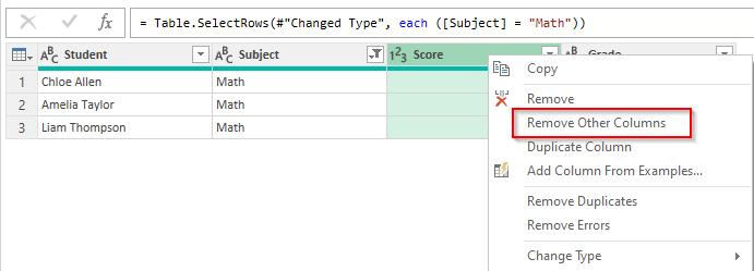
➤ Select the column with the return range/lookup array and click on the column header. Right-click and choose Remove Other Columns.
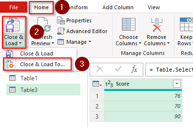
➤ As Excel keeps the matching cells for the given criteria, go to the Home tab and click on Close & Load >> Close & Load To.
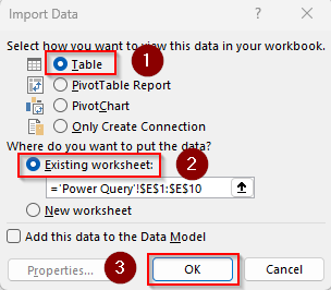
➤ Choose Table and Existing Worksheet or New Worksheet as you prefer.
➤ Here’s the final result:
Custom VBA Macro to Return Multiple Values Based on Single Criteria
Customizing a VBA Macro allows you to return multiple values based on single criteria in any format you want. All you need to do is define the criteria and lookup range.
You can put the returned values in a column, row, or a single cell. For this, follow the steps given below:
➤ To add the Developer tab in the top ribbon, go to the File tab >> More >> Options.
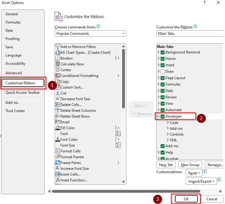
➤ Click on Customize Ribbon, check the Developer box, and press Ok.
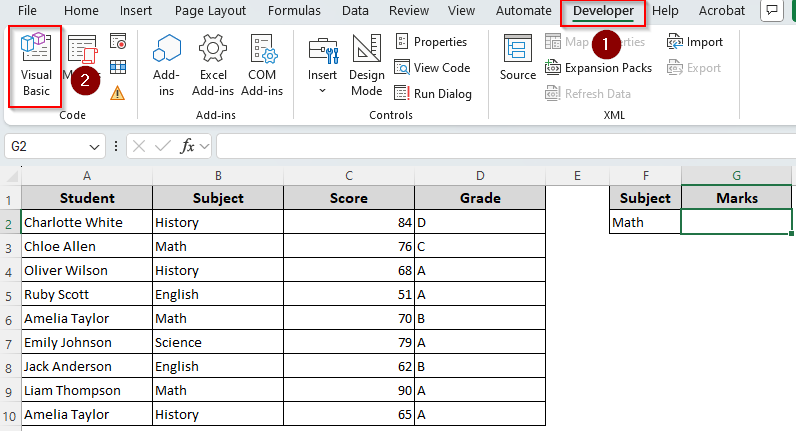
➤ Now, go to the Developer tab and click on Visual Basic.
➤ When the VBA Editor opens, click Insert and choose Module.
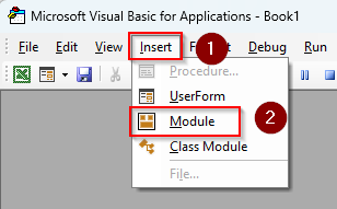
➤ In the blank module box, insert the following code:
Sub Return_Multiple_Values()
Dim criteria As Variant
Dim lookupRange As Range
Dim returnRange As Range
Dim matchType As String
Dim resultValues As Collection
Dim i As Long
Dim result As String
Dim outputCell As Range
' Step 1: Get user input
criteria = InputBox("Enter the lookup value (e.g., 'Math') or a reference (e.g., F2):")
If criteria = "" Then Exit Sub
On Error Resume Next
Set lookupRange = Application.InputBox("Select the lookup range (e.g., column B):", Type:=8)
If lookupRange Is Nothing Then Exit Sub
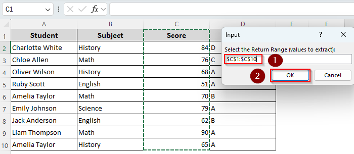
Set returnRange = Application.InputBox("Select the return range (e.g., column C):", Type:=8)
If returnRange Is Nothing Then Exit Sub
On Error GoTo 0
If lookupRange.Rows.Count <> returnRange.Rows.Count Then
MsgBox "Lookup and return ranges must be of the same size.", vbExclamation
Exit Sub
End If
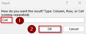
matchType = Application.InputBox("How do you want the result? Type: Column, Row, or Cell (comma-separated):", Type:=2)
matchType = LCase(Trim(matchType))
If matchType <> "column" And matchType <> "row" And matchType <> "cell" Then
MsgBox "Invalid option. Please enter Column, Row, or Cell.", vbExclamation
Exit Sub
End If
' Step 2: Find matching values
Set resultValues = New Collection
For i = 1 To lookupRange.Cells.Count
If StrComp(CStr(lookupRange.Cells(i).Value), CStr(criteria), vbTextCompare) = 0 Then
resultValues.Add returnRange.Cells(i).Value
End If
Next i
If resultValues.Count = 0 Then
MsgBox "No matching values found.", vbInformation
Exit Sub
End If
' Step 3: Output results
Set outputCell = Application.InputBox("Select the first output cell:", Type:=8)
If outputCell Is Nothing Then Exit Sub
If matchType = "column" Then
For i = 1 To resultValues.Count
outputCell.Offset(i - 1, 0).Value = resultValues(i)
Next i
ElseIf matchType = "row" Then
For i = 1 To resultValues.Count
outputCell.Offset(0, i - 1).Value = resultValues(i)
Next i
ElseIf matchType = "cell" Then
result = ""
For i = 1 To resultValues.Count
result = result & resultValues(i) & ", "
Next i
result = Left(result, Len(result) - 2) ' Remove trailing comma
outputCell.Value = result
End If
MsgBox "Done! Returned " & resultValues.Count & " values.", vbInformation
End Sub
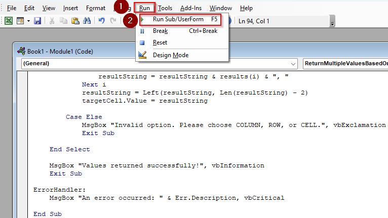
➤ Press F5 to run the code or click on the Run tab >> Run Sub/UserForm.
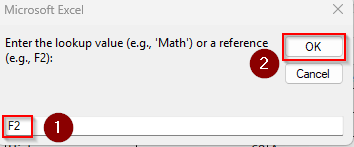
➤ Now, enter a value or cell reference to match and press Ok.
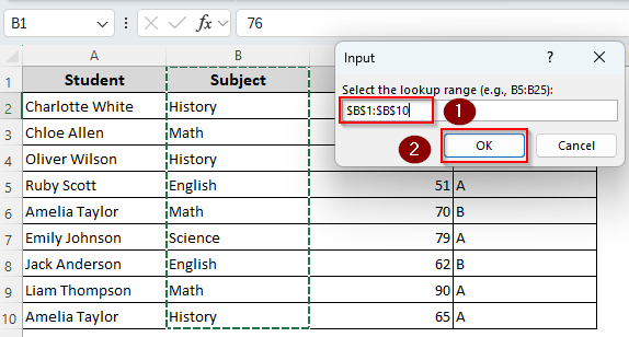
➤ As Excel prompts you to select the lookup range, go back to the Excel tab and highlight or manually type the range. Click Ok.
➤ Similarly, highlight or type the return range manually and press OK.
➤ Select how you want your returned values. Choose Column, Row, or Cell (Separated by Comma) as needed. Press Ok.
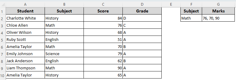
➤ Here’s the final result for our dataset:
Frequently Asked Questions
How to return multiple unique values based on a single criterion?
To return multiple unique values matching a criterion, you can combine the FILTER and UNIQUE functions. Enter the following formula in a blank cell:
=UNIQUE(FILTER(C1:C10, B1:B10=F2))
Change the return range C1:D10, criteria range B1:B10, and criteria F2 according to your dataset.
How to return custom texts for no matches based on criteria?
If you want it to return a custom text such as No Match Found, use the following formula:
=IFERROR(TEXTJOIN(“,”, TRUE, FILTER(C1:C10, B1:B10=F2)), “No Match Found”)
Change the ranges and criteria as needed. Also, if you want to results in an array instead of joining them with commas, use this formula:
=IFERROR(FILTER(C1:C10, B1:B10=F2), “No Match Found”)
How do I return all values that match multiple criteria in Excel?
Select a cell to put the first match and insert the following formula:
=IFERROR(INDEX(C1:C10, SMALL(IF((B1:B10=”Math”)➤(C1:C10=”Science”), ROW(B1:B10)-ROW(B1)+1), ROW(1:1))), “”)
Change the return range, criteria range, and criteria as needed and press CTRL + SHIFT + ENTER for old Excel versions or Enter for the new ones.
Concluding Words
Although using the FILTER function is the easiest way to return a spill range of matched values, it’s not available in old Excel versions. Therefore, you need to use a combination of INDEX, SMALL, and ROW functions to achieve similar results.
However, the TEXTJOIN and IF functions work in all Excel versions if you want to join all the matches in a single cell. Choose the formulas based on whether you want an array of matched values in a column, row, or cell.


i am having problems finding help for my particular problem
say i have columns a, b and c
column a is a date, column b is a store name, column c needs to have a date that is x days after the column A based on which of 7 stores is in column b.
im assuming it’s an ifs statement, and a sum statement but i can’t seem to get the coding right.
Hello Lee,
Instead of creating a long nested IFS, you can use a clean lookup table. Create a small table somewhere (e.g., E2:F8):
| Store | Days |
| —— | —- |
| Store1 | 5 |
| Store2 | 10 |
| Store3 | 7 |
| Store4 | 3 |
| Store5 | 14 |
| Store6 | 2 |
| Store7 | 21 |
Then use XLOOKUP: =A2 + XLOOKUP(B2, E2:E8, F2:F8)
or for VLOOKUP: =A2 + VLOOKUP(B2, E2:F8, 2, FALSE)
Please let us know if you need further assistance.
What would the code look like to search a column of numbers (ie.lookupRange) and to return all values in that column (ie.lookupRange) that could add up to a known value. Example a column has the numbers 26, 36 and 48, 60. I then have another column (ie.returnRange) that lists the remaining value/number if the values from the lookupRange (ie. 26, 36 and 48, 60) are subtracted from 96 (so that column has 70, 60, 48, and 36 thus the returnRange). For each value in the returnRange, the code will return all values from the lookupRange that can be added to the cell values in the returnRange to equal a grand total of 96 or less. So for returnRange value of 70 it will only return 26 (equals a total of 96). For a value of 60 it will return 26 and 36 (each can be added to 60 and be equal to or less than 96). And Etc.
Hello John,
Use the FILTER function. For a return value in C2 and lookup values in A2:A5, use
=FILTER(A2:A5, A2:A5 + C2 <= 96) This returns all numbers from the lookup range that can be added to the return value without exceeding 96.