When working with large datasets, finding and managing rows with similar values can be challenging. Instead of manually sorting or filtering, you can group rows by cell values in Excel. Grouping helps you summarize, organize, and analyze data efficiently without losing important details.
In this article, we’ll cover four practical methods to group rows by cell value using the Data tab, Pivot Tables, Power Query, and the GROUPBY function in Excel 365. Let’s get started.
Steps to group rows by cell value in Excel:
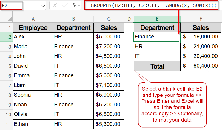
➤ Select a blank cell where you want the grouped summary to appear such as E2.
➤ Enter the following formula:
=GROUPBY(B2:B11, C2:C11, LAMBDA(x, SUM(x)))
Here, B2:B11 is the Department column used for grouping, C2:C11 is the Sales column to be aggregated, and LAMBDA applies the SUM function to total sales within each department.
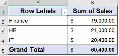
➤ Press Enter and Excel will generate a dynamic array showing each department with its total sales. Optionally, format your data as you prefer.
Insert the GROUPBY Function to Summarize Rows by Cell Value
For users of Excel 365 or Excel Online, the GROUPBY function offers a modern and efficient way to summarize data without relying on Pivot Tables or Power Query. This dynamic formula allows you to group rows based on a column and apply aggregation functions like SUM, AVERAGE, or COUNT, all in a single step. The output goal here is to quickly generate a compact summary showing total sales per department directly in a cell range, saving time and avoiding manual calculations. Here, the goal is to group rows by the Department column to better understand performance across HR, Finance, and IT.
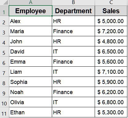
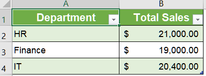
We’ll use the following dataset for demonstration:
Steps:
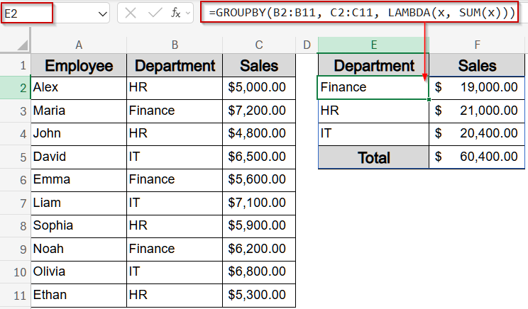
➤ Select a blank cell where you want the grouped summary to appear such as E2.
➤ Enter the following formula:
=GROUPBY(B2:B11, C2:C11, LAMBDA(x, SUM(x)))
Here, B2:B11 is the Department column used for grouping, C2:C11 is the Sales column to be aggregated, and LAMBDA applies the SUM function to total sales within each department.
➤ Press Enter and Excel will generate a dynamic array showing each department with its total sales. Optionally, format your data as you prefer.
This method is ideal for users who want a quick, formula-driven summary without dealing with Pivot Tables or loading data into Power Query.
Note:
The GROUPBY function is only available in the latest Excel versions.
Organize Rows by Cell Value Using the Data Tab
When you want to make your dataset easier to navigate without using formulas or advanced tools, the Group feature in Excel’s Data tab provides a straightforward way to organize rows. This approach is especially useful when your dataset is sorted by the column you intend to group, such as Department. By grouping rows together, you can quickly expand or collapse sections of data, which improves readability and makes comparisons much easier.
The output goal here is to create collapsible groups of rows based on Department values, allowing you to hide or show entire categories with a single click.
Steps:
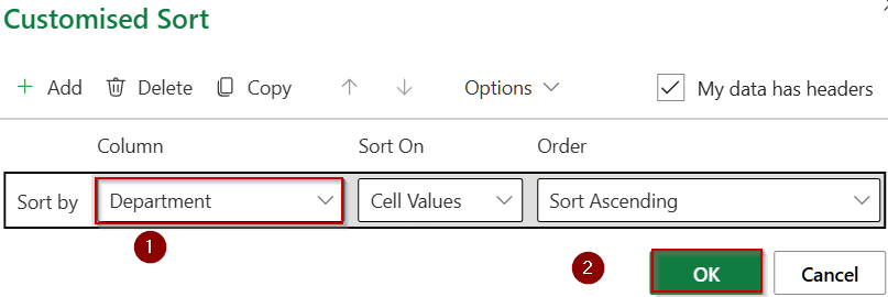
➤ First, sort your data by the Department column. Go to the ribbon, click Data >> Sort, and choose Department.
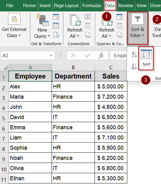
➤ Under Sort by, choose Department and click OK.
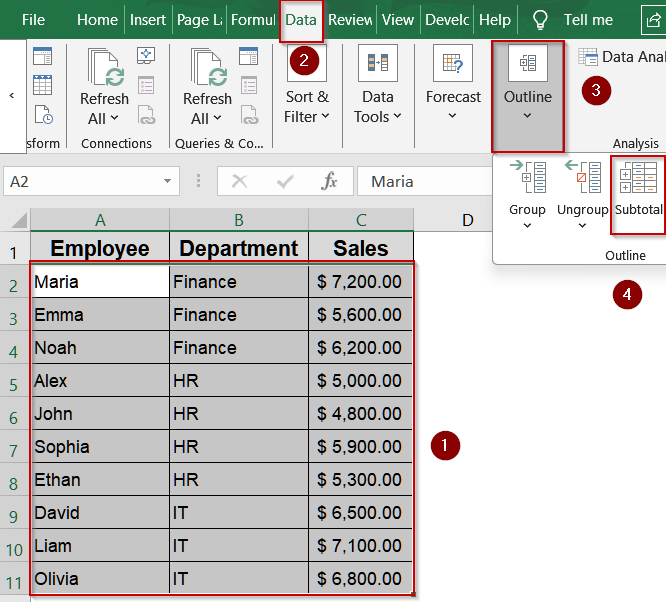
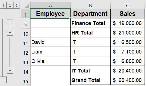
➤ Go to the Data tab >> Click on Outline >> Select Subtotal.
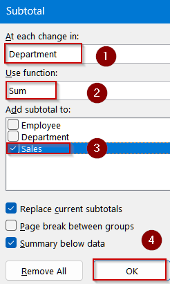
➤ In the dialog, select Department under At each change in, set Use Function to Sum and check Sales under Add subtotal. Then, click OK.
➤ Now, you’ll see a minus/plus sign on the left side of the sheet, allowing you to expand or collapse grouped rows by department.
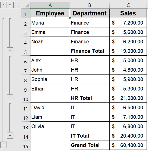
This simple yet powerful technique ensures your dataset looks cleaner while helping you focus on one department’s data at a time.
Summarize Rows by Cell Value Using a Pivot Table
If you’re working with larger datasets or need a more analytical view, Pivot Tables provide a dynamic way to group and summarize data in Excel. Unlike manual grouping, Pivot Tables not only organize rows but also allow you to calculate totals, averages, counts, or even the highest and lowest values per category. This flexibility makes them ideal for reporting, analysis, and quick decision-making.
The output goal here is to generate a compact summary showing department-wise totals or other calculations without altering the original dataset.
Steps:
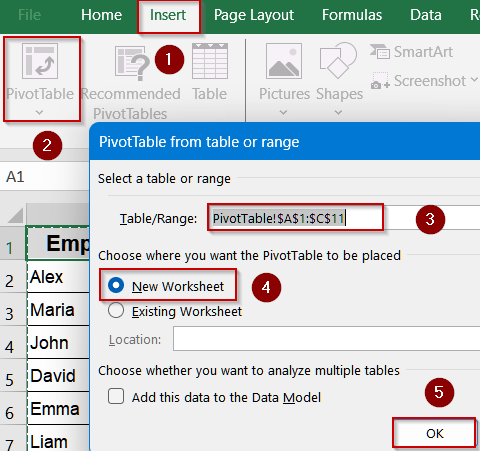
➤ Select your dataset and go to Insert >> PivotTable. Confirm your range and select New Worksheet to place your PivotTable >> Click OK.
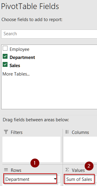
➤ In the PivotTable Field List, drag Department into the Rows area.
➤ Drag Sales into the Values area. By default, it will display the sum of sales for each department.
➤ If needed, adjust the summary calculation by clicking the drop-down in Values and selecting options like Average, Count, or Max.
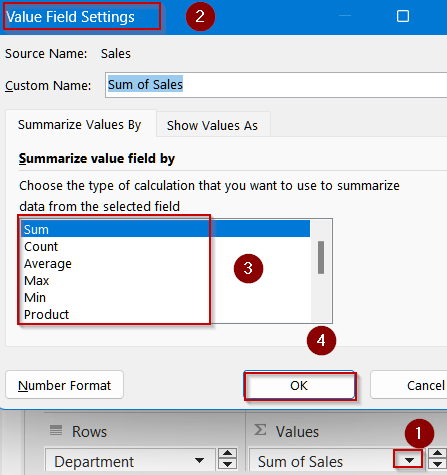
➤ You’ll now have a grouped report that displays total (or other chosen metrics) by department, neatly summarized in a Pivot Table.
This method is excellent for anyone needing quick summaries or department-level insights without manually grouping and calculating.
Use Power Query to Group Rows by Cell Value
When working with large datasets or recurring reporting tasks, Power Query offers a powerful way to automate data transformation and grouping in Excel. Unlike manual grouping or Pivot Tables, Power Query allows you to create repeatable workflows, apply multiple aggregation functions, and handle complex datasets efficiently. It’s perfect for users who want a clean, organized summary without manually altering the original data. The output goal here is to generate a concise table showing department-wise totals of sales, ready to be loaded back into Excel for reporting or analysis.
Steps:
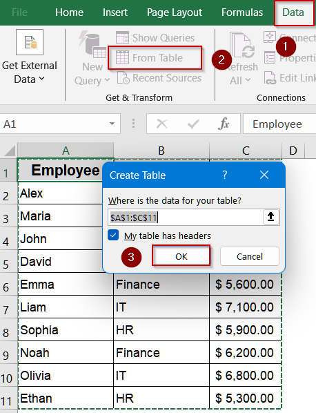
➤ Select your dataset and go to Data tab >> Get & Transform >> From Table/Range and click OK to load it into Power Query.
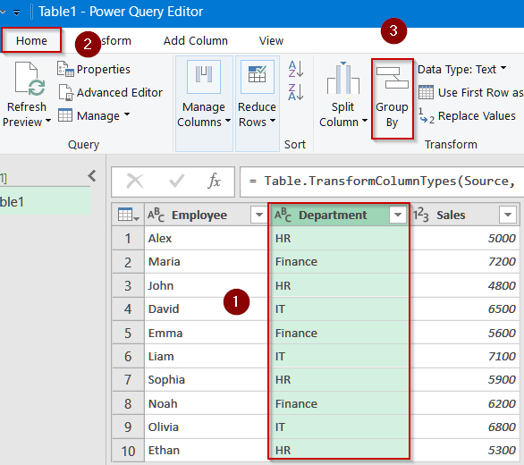
➤ In the Power Query Editor, select the Department column.
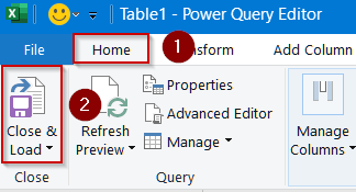
➤ Go to Home tab >> Group By. A dialog box will appear.
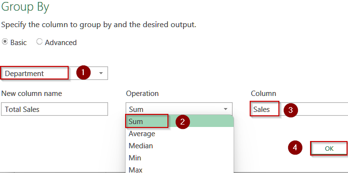
➤ In the Group By window, set Department as the grouping column. Under Operations, select Sum for the Sales column. You can also choose other aggregations like Average or Count if needed.
➤ Click OK, and Power Query will generate a grouped table showing total sales per department.
➤ Finally, click Close & Load to insert the summarized result back into Excel.
This method is ideal for advanced users who frequently handle large datasets and want a repeatable, automated solution for summarizing department-level totals efficiently.
Frequently Asked Questions
Can I group rows by cell value without a Pivot Table in Excel?
Yes, you can. Excel offers grouping through the Data tab, Power Query, and even formulas like GROUPBY function in Microsoft Office 365, which helps aggregate data directly without a Pivot Table.
Why is Power Query better for grouping rows than manual methods?
Power Query is dynamic and refreshable. Once you load your dataset into Power Query and define grouping rules, you can update results instantly when new data is added, saving time for recurring reports.
Does the GROUPBY function work in all Excel versions?
No, the GROUPBY function is part of the newer Excel versions that support dynamic arrays and advanced formulas. Older versions like Excel 2016 or 2013 won’t recognize this function.
What’s the advantage of grouping rows using Pivot Tables?
Pivot Tables allow quick summarization, filtering, and grouping without altering raw data. They are flexible, easy to update, and widely used for analyzing datasets with multiple categories and numerical values.
Wrapping Up
In this tutorial, we explored four practical methods to group rows by cell value in Excel. Each method has its own strength starting from simple grouping with Data tab, quick summaries with Pivot Tables, advanced reshaping with Power Query, and formula-driven grouping with Excel 365 functions. Choosing the right approach depends on your dataset size, reporting needs, and Excel version. Feel free to download the practice file and share your feedback.