In Excel, creating a new table based on data from an existing table is a common task. This can help summarize, reorganize, or extract relevant information efficiently. Instead of manually copying data, Excel offers multiple methods to generate a new table dynamically using formulas or functions.
In this article, we will explore three effective ways to create a table from another table in Excel. Each method is explained step by step, making it easy for beginners and advanced users alike to implement.
Steps to create a table from another table in Excel:
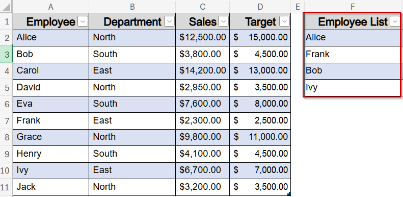
➤ In F2:F5, list the employees for your new table such as Alice, Frank, Bob, and Ivy. Then, select range and press Ctrl + T to turn it into a table.
➤ In G2, enter the following formula to get the Sales value:
=INDEX($C$2:$C$11, MATCH(L2, $A$2:$A$11, 0))
Here, MATCH function finds the row number of the employee name within the original table, and INDEX function retrieves the corresponding Sales value from column C.
➤ Press Enter, then drag the formula down to fill all rows in G2:G6.

Extract and Filter Data from Multiple Columns into a New Table
If you’re working with a large dataset and need to extract specific records like grouping employees by department, then extracting data from multiple columns using INDEX, IF, and SMALL functions is an efficient solution. This approach allows you to dynamically create a separate, organized table from existing data without manual filtering or copying.
We’ll use the dataset below to find the employee names working in specific regions like North and South.

Steps:
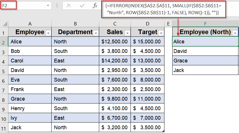
➤ Select cell F2 in the new table.
➤ Enter the following formula:
=IFERROR(INDEX($A$2:$A$11, SMALL(IF($B$2:$B$11="North", ROW($B$2:$B$11)-1, FALSE), ROW()-1)), "")
Here, INDEX returns the Employee Name, IF finds rows where the Department is North and SMALL ensures the nth matching employee is returned in sequence.
➤ Press Ctrl + Shift + Enter if you are using Excel 2019 or earlier (for array formulas). In Excel 365 or 2021, simply press Enter .
➤ Use the Fill Handle to drag the formula down to cover all possible North employees if the names aren’t filled in automatically.
➤ Enter this formula in G2 cell to fetch the names for employees working in the South department:
=IFERROR(INDEX($A$2:$A$11, SMALL(IF($B$2:$B$11="South", ROW($B$2:$B$11)-1, FALSE), ROW()-1)), "")
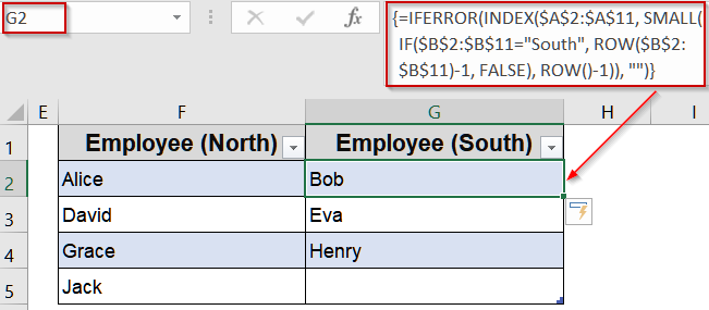
Now we have a new table created from our existing table.
Insert INDEX and MATCH Functions for a Flexible Lookup
When you need to dynamically retrieve values like Sales based on employee names, INDEX and MATCH is a powerful alternative to VLOOKUP. Unlike VLOOKUP, this combination allows you to look up values from any column and is more robust when your data structure changes. Here, we’ll create a new table that lists selected employees such as Alice, Frank, Bob, and Ivy and retrieves their corresponding Sales values from the master dataset. This method is especially useful for dashboards or reports that need flexible lookups without rearranging your columns.
Steps:
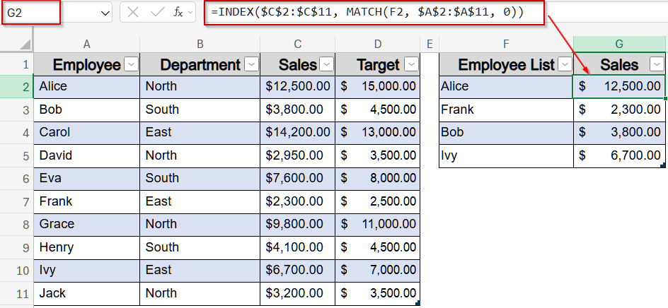
➤ In F2:F5, list the employees for your new table such as Alice, Frank, Bob, and Ivy. Then, select range and press Ctrl + T to turn it into a table.

➤ In G2, enter the following formula to get the Sales value:
=INDEX($C$2:$C$11, MATCH(L2, $A$2:$A$11, 0))
Here, MATCH function finds the row number of the employee name within the original table, and INDEX function retrieves the corresponding Sales value from column C.
➤ Press Enter, then drag the formula down to fill all rows in G2:G6.
This approach is dynamic, adaptable to column changes, and perfect for scenarios where you need reliable lookups without depending on fixed column positions.
Apply VLOOKUP Function to Retrieve Corresponding Data
If you want to extract related columns such as Sales and Target for only a few selected employees from a larger dataset, VLOOKUP function is one of the simplest and most dependable options. It eliminates the need to manually search through rows by automatically fetching values for the employees you specify. In this case, we’ll create a compact table showing only Alice, Frank, Bob, and Ivy, along with their Sales and Target values from the master list. This method is perfect for creating focused dashboards or filtered reports without clutter.
Steps:
➤ In F2:F5, list the employees for your new table such as Alice, Frank, Bob, and Ivy. Then, select range and press Ctrl + T to turn it into a table.
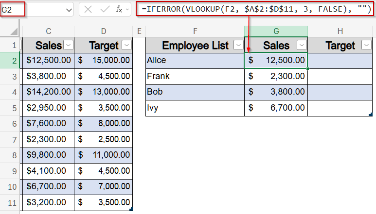
➤ In G2, enter this formula to get Sales:
=IFERROR(VLOOKUP(F2, $A$2:$D$11, 3, FALSE), "")
Here, VLOOKUP searches for each name in F2:F5 within A2:D11. Column index 3 retrieves Sales and the FALSE argument enforces exact matches, while IFERROR hides errors by returning blank cells for missing names.
➤ In H2, enter this formula to get Target:
=IFERROR(VLOOKUP(F2, $A$2:$D$11, 4, FALSE), "")
Here, column index 4 retrieves value for Target.
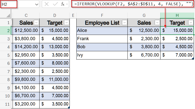
The formula will spill automatically in our new table.
Frequently Asked Questions
Can I create a new table that updates automatically when the original table changes?
Yes. Using formulas like VLOOKUP with COLUMN or INDEX-MATCH allows the new table to remain dynamically linked to the original table, so any changes in the source table are instantly reflected in the new table.
Which method is best for combining multiple columns into one table?
Merging multiple columns using concatenation is simple and effective when you want to combine values in a readable format. It is ideal for summarizing data or creating unique identifiers without affecting the original table structure.
Can INDEX-MATCH functions be used if the lookup column is not the first column?
Yes. The INDEX and MATCH formula is more flexible than VLOOKUP because it allows you to retrieve data from any column, regardless of its position, ensuring accuracy even if the table’s layout changes.
Is it possible to create a new table without formulas?
Yes. You can manually copy and paste the data as values or use Power Query to extract and transform the original table into a new table without relying on formulas.
Can I combine multiple methods for creating a table from another table?
Yes. You can merge columns for readability, use functions like VLOOKUP for dynamic updates, and INDEX-MATCH for flexibility. Combining these methods allows you to create tables tailored to different reporting or analytical requirements.
Wrapping Up
In this tutorial, we explored three efficient ways to create a new table from another table in Excel. By using functions like INDEX with SMALL, VLOOKUP, or INDEX with MATCH, you can automate table creation, save time, and maintain accuracy. These methods are ideal for summarizing large datasets, generating reports, or restructuring data dynamically. Feel free to download the practice file and share your feedback.