Mirroring a table on another sheet is a powerful way to keep your data synchronized across multiple locations. Whether you’re building dashboards, reports, or summary sheets, having a mirrored table ensures that updates in the original dataset automatically reflect in the linked table. This avoids manual duplication and reduces errors.
In this article, we’ll explore four effective methods to mirror a table in Excel, ranging from simple formulas to Power Query, conditional formulas, and VBA automation. Each method comes with step-by-step instructions and a sample dataset so you can replicate the process easily.
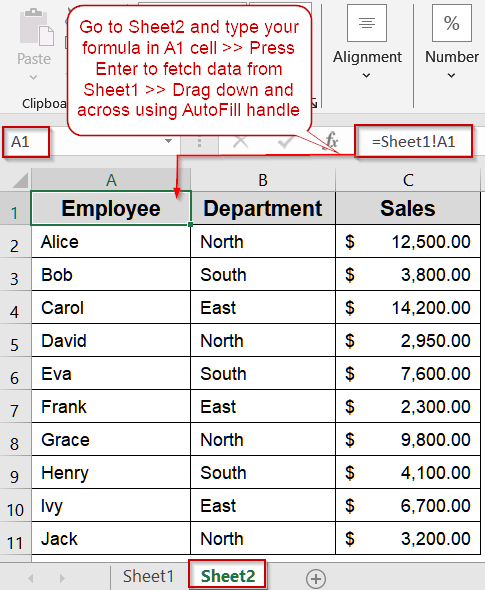
Steps to mirror table on another sheet in Excel:
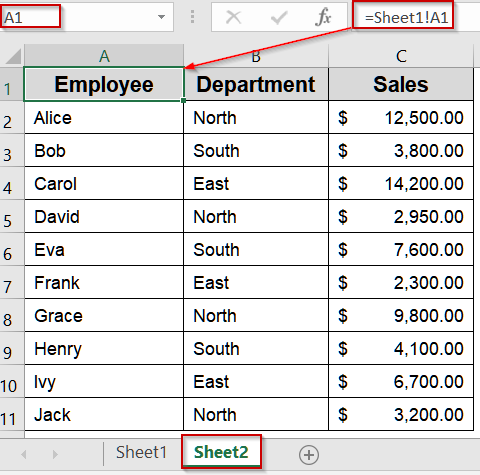
➤ Go to the sheet where you want to create the mirrored table (e.g., Sheet2).
➤ In cell A1, type formula: =Sheet1!A1
➤ Press Enter for output.
➤ Drag the formula across all columns and down for all rows in your table.
Link the Original Table Using Simple Formulas
For small datasets, the easiest way to mirror a table is to link each cell in the new sheet directly to the original table using formulas. This method ensures that any updates in the original table reflect automatically in the mirrored table. It’s ideal for quick dashboards or summary sheets with a limited number of columns.
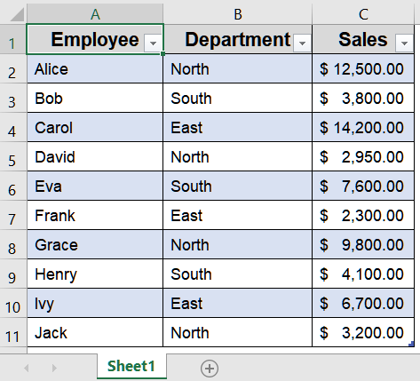
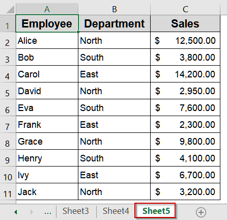
This is the original table in Sheet1 that we will mirror:
Steps:
➤ Go to the sheet where you want to create the mirrored table (e.g., Sheet2).
➤ In cell A1, type formula:
=Sheet1!A1
➤ Press Enter for output.
➤ Drag the formula across all columns and down for all rows in your table.
Now, your Sheet2 table will dynamically mirror the data in Sheet1. Any changes in Sheet1 will immediately appear in Sheet2.
Apply Conditional Formula to Mirror an Entire Table
Sometimes, you may want to mirror a table on a different sheet so that any updates in the original table are reflected automatically. By using a formula with INDEX and IF functions, you can replicate the full table on another sheet without manually copying the data.
Steps:
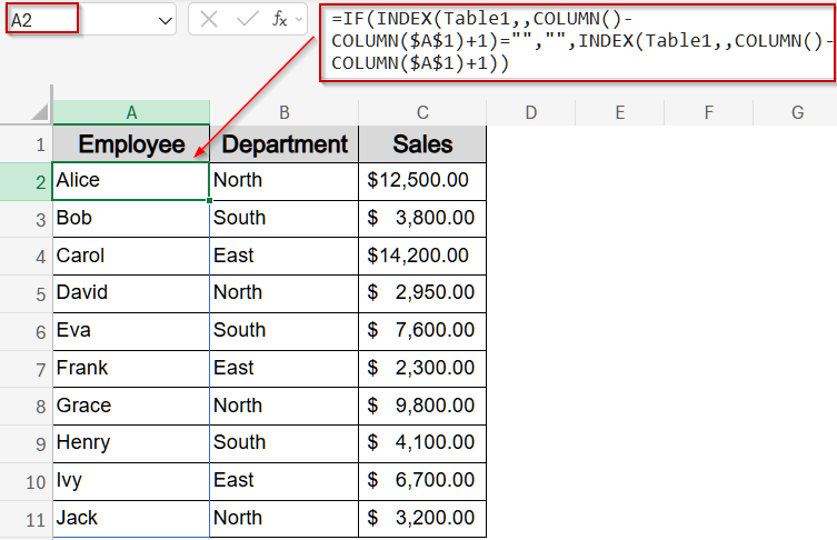
➤ In Sheet3, select the first cell where you want mirrored data such as A2.
➤ Enter a formula like:
=IF(INDEX(Table1,,COLUMN()-COLUMN($A$1)+1)="","",INDEX(Table1,,COLUMN()-COLUMN($A$1)+1))
This formula mirrors the entire Table1 by dynamically referencing columns relative to the starting cell $A$1. INDEX function pulls the column data, and IF function leaves the cell blank if the value is empty.
➤ Press Ctrl + Shift + Enter for array formulas (Excel 2019 or earlier).
➤ Drag across and down to fill the mirrored table.
Now, the data from the table is fully mirrored on a different sheet.
Use Power Query to Mirror a Table on Another Sheet
Power Query allows you to import and transform your original dataset and load it into another sheet. This is especially useful for larger datasets or when you want to filter, sort, or shape data before mirroring. Let’s see how to get the job done.
Steps:
➤ Open the sheet with your main table such as Sheet1.
➤ Go to the Data tab and select Get Data >> From Other Sources >> From Table/Range.
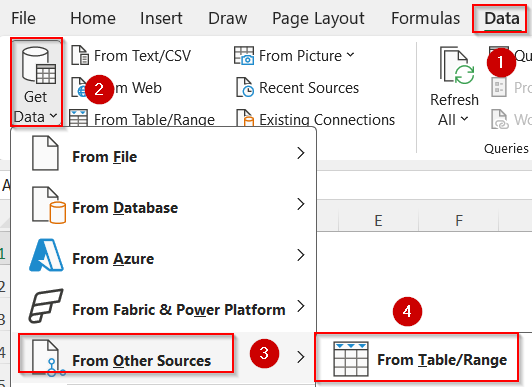
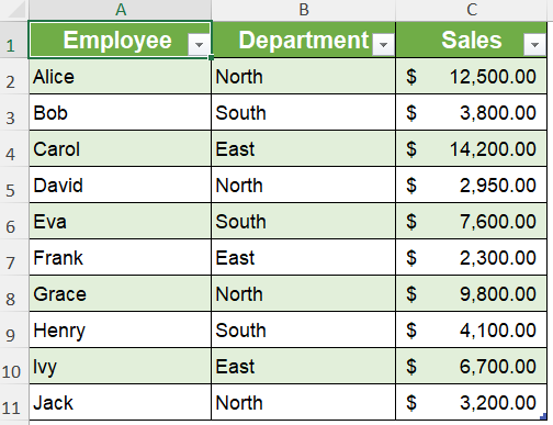
➤ Your table will automatically load it into the Power Query Editor.
➤ In the Power Query Editor, you can choose which columns to keep, filter rows, or sort data as needed.
➤ Once your data is ready, click Close & Load from the Home tab to display the mirrored table on another sheet such as Sheet4.

This creates a dynamic mirrored table that automatically updates whenever the source data changes, giving you a flexible way to manage and reflect your dataset.
Mirror a Table Automatically Using VBA Code
For large datasets or repetitive tasks, VBA can automate the mirroring process completely. You can write a macro that copies the table from one sheet to another whenever the data updates.
Steps:
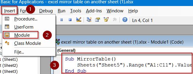
➤ Press Alt + F11 to open the VBA editor.
➤ Insert a new module and paste the following code:
Sub MirrorTable()
    Sheets("Sheet5").Range("A1:C11").Value = Sheets("Sheet1").Range("A1:C11").Value
End Sub
➤ Close the editor and run the macro by pressing F5 Key.
This instantly copies the original table to Sheet5. You can also assign it to a button for quick refresh.
Note:
If your data appears unformatted, you need to format it manually.
Frequently Asked Questions
Can I mirror only part of the table?
Yes. By using conditional formulas, such as INDEX and IF, or Power Query, you can mirror only certain rows or columns based on specific criteria like Department, Region, or Sales. This creates a filtered mirrored table automatically.
Will mirrored tables update automatically?
Formulas and Power Query connections update automatically whenever the source data changes. VBA macros, however, only refresh the mirrored table when executed or triggered by an event, so they may require manual or programmed updates to stay synchronized.
Can I mirror a table to multiple sheets at once?
Yes. You can copy the linking formulas across multiple sheets, or adjust a VBA macro to loop through all desired sheets. This allows simultaneous updates in several mirrored tables whenever the original table changes.
Is it possible to preserve formatting in the mirrored table?
Formulas only mirror values, not cell formatting. To maintain formatting along with data, you can use VBA to copy both content and styles from the source table, ensuring that the mirrored table visually matches the original sheet.
Which method is best for large datasets?
For large datasets, Power Query and VBA are preferred because they handle many rows efficiently and allow automation. Using formulas for large tables can slow down Excel and may require extra steps to maintain performance.
Wrapping Up
In this tutorial, we explored four practical methods to mirror a table on another sheet in Excel, including linking formulas, Power Query, conditional formulas, and VBA. Each approach allows you to keep your mirrored table synchronized automatically or on demand. By applying these techniques, you can create dynamic dashboards, filtered reports, or summaries without manually copying data. Feel free to download the practice file and share your feedback.