Structured reference in Excel is a way to refer to table data by column names instead of cell references. When you convert a range into an Excel Table, Excel allows you to write formulas like =SUM(Sales[Revenue]) instead of =SUM(C2:C11). This makes formulas easier to read, understand, and update.
Structured references are especially useful when working with dynamic tables. If you add new rows or rename columns, formulas with structured references update automatically without needing any manual changes.
In this article, you’ll learn how to use structured references in Excel formulas step by step with examples.
Here’s how structured references work in Excel:
➤ Open your dataset in Excel.
➤ Click on any cell in the table to activate the Table Design tab in the Ribbon.
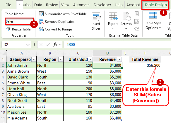
➤ Go to the Table Design tab and rename the table to Sales in the Table Name field.
➤ Now, click on cell F2 where you want to calculate the total revenue
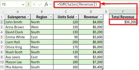
➤ Enter this formula =SUM(Sales[Revenue])
➤ Press Enter. Excel will instantly calculate the total of the Revenue column from the Sales table.
Use Structured Reference with the SUM Function
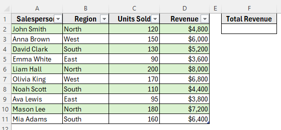
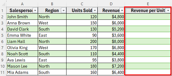
In the following dataset, we have monthly sales data as a table format. Column A lists the Salesperson names, Column B shows their Region, Column C contains Units Sold, and Column D lists the Revenue earned. Column F is empty, outside of the table, where we’ll enter formulas using structured references to display Total Revenue.
We’ll use this dataset to demonstrate different ways to use structured references in Excel formulas.
One of the most common ways to use structured references in Excel is with the SUM function. Instead of writing a formula using traditional cell references like =SUM(D2:D11), you can refer to the column by its name, which makes your formula much easier to read and maintain.
Structured references automatically adjust when you add new rows or rename a column.
Here’s how to do it step by step:
➤ Open your dataset in Excel.
➤ Click on any cell in the table to activate the Table Design tab in the Ribbon.
➤ Go to the Table Design tab and rename the table to Sales in the Table Name field.
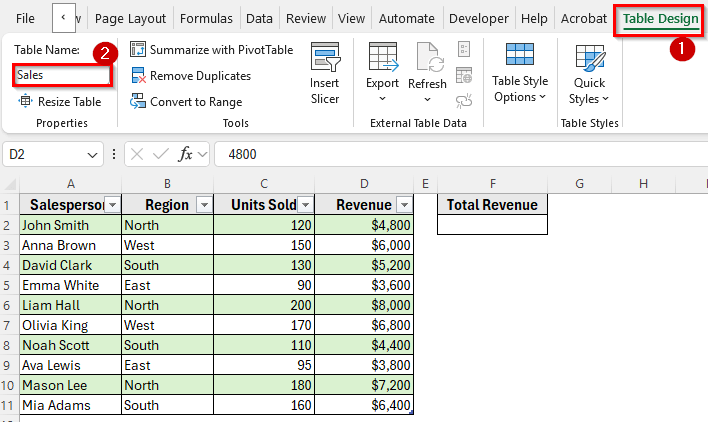
➤ Now, click on cell F2 where you want to calculate the total revenue.
➤ Enter this formula:
=SUM(Sales[Revenue])
➤ Press Enter. Excel will instantly calculate the total of the Revenue column from the Sales table.
➤ If you add new rows to the table, this formula will update automatically without needing any changes.
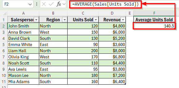
Applying AVERAGE Function to Use Structured Reference
You can also use structured references with the AVERAGE function to calculate the average of a column without using traditional cell references.
Here’s how:
➤ Add a new column outside of the table in Column F and name it Average Units Sold. This is where we’ll calculate the average number of units sold.
➤ Click on cell F2 and enter the formula below:
=AVERAGE(Sales[Units Sold])
➤ Press Enter.
➤ Excel will return the average units sold from the Units Sold column.
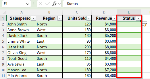
Apply Structured Reference with the IF Function for Conditional Results
Structured references also work perfectly with logical formulas like IF, which is useful when you want to evaluate conditions row by row. For example, you can check if each salesperson sold more than 150 units.
Here’s how to do it step by step:
➤ Open your dataset in Excel.
➤ Add a new column to the table in Column E and name it Status. This is where we’ll display whether each salesperson met the target or not.
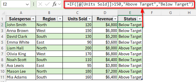
➤ Click on cell E2 and enter the following formula:
=IF([@[Units Sold]]>150,"Above Target","Below Target")
➤ Press Enter. Excel will show Above Target if the salesperson sold more than 150 units, and Below Target if they didn’t.
Use Structured Reference with VLOOKUP
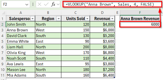
Structured references can also be combined with lookup functions. For example, if you want to find the revenue of a specific salesperson, you can use the VLOOKUP function.
Here’s how to do it:
➤ Add a new column outside of the table in Column F and name it Anna Brown Revenue.
➤ Click on cell F2 where we’ll calculate the total revenue of this specific salesperson.
➤ Enter the formula below:
=VLOOKUP("Anna Brown", Sales, 4, FALSE)
➤ Press Enter. Excel will return Anna Brown’s revenue from the Revenue column.
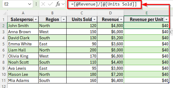
Use Structured Reference for Calculations Across Multiple Columns
One of the biggest advantages of structured references is how clean and readable they make formulas when performing calculations across multiple columns. By this method, you can calculate Revenue per Unit for each salesperson by dividing the total revenue by the number of units sold.
Here’s how to apply this method:
➤ Add a new column to the table in Column E and name it Revenue per Unit. This column will display how much revenue each unit generated.
➤ Click on cell E2 and enter the following formula:
=[@[Revenue]]/[@[Units Sold]]
➤ Press Enter. Excel will calculate the revenue per unit for the entire column.
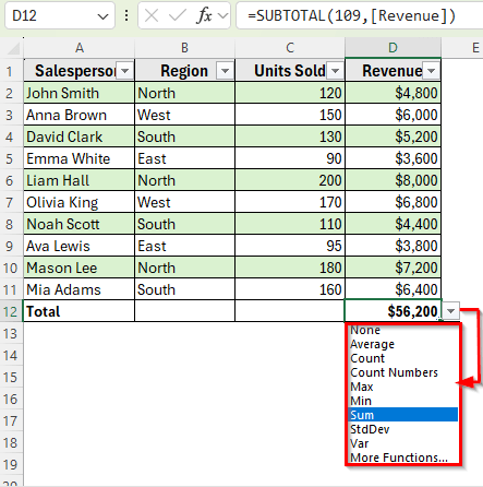
Enable Total Row to Use Structured References Automatically
Another practical way to use structured references in Excel is by enabling the Total Row in a table. When you turn this feature on, Excel automatically uses structured references in the formulas it inserts.
Here’s how to do it step by step:
➤ Click anywhere inside the table to activate the Table Design tab on the ribbon.
➤ In the Table Style Options group, check the Total Row box. Excel will instantly add a new row at the bottom of your table.
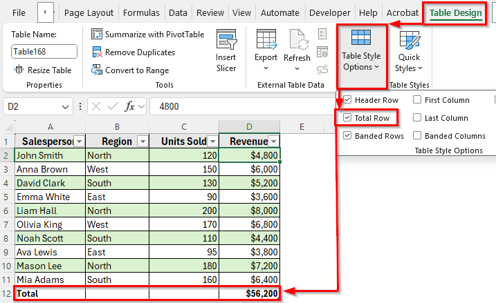
➤ By default, Excel displays a SUM for the last numeric column such as Revenue. If it doesn’t, click the cell under the Revenue column in the Total Row, open the drop-down list, and select Sum.
➤ The formula will appear automatically as a structured reference, like this:
=SUBTOTAL(109, Sales[Revenue])
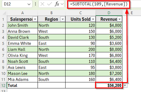
➤ You can change the calculation type to Average, Count, Max, or Min by selecting them from the drop-down list. Excel will automatically adjust the formula using structured references.
Frequently Asked Questions
How to use a structured reference in a formula in Excel?
To use a structured reference in a formula, you first need to convert your dataset into a table. Then calculate the total of the Revenue column in a table named Sales, use a structured reference in this following formula:
=SUM(Sales[Revenue])
Press Enter. Excel will calculate the total revenue from the Revenue column.
What does @ mean in structured references?
The @ symbol refers to the current row within a structured reference. For example, [@[Revenue]] refers to the Revenue value in the same row.
Can I use structured references outside the table?
Yes. You can use them anywhere in your workbook by typing the table name followed by the column name in square brackets.
Wrapping Up
Structured references in Excel make formulas more readable, flexible, and easier to maintain. They automatically update when you add rows, rename columns, or expand your dataset.
You can use them with functions like SUM, AVERAGE, IF, VLOOKUP, or even custom calculations. Once you start using structured references, your formulas will become more self-explanatory.