
Creating a search box in Excel makes it easier for users to quickly locate and display specific data within a dataset without needing to scroll manually. Using Excel’s built-in tools and functions, we can easily create a search box to find, filter, and display specific data from a dataset.
Follow the steps below to create your own search box within an Excel worksheet:
➤ In your dataset, go to the cell where you want the search result to appear and enter the formula:
=FILTER(array, include, [if_empty])
➤ Replace “array” with the range of cells where you want to return the results from.
➤ Replace “include” with the condition or criteria that determines which rows to return.
➤ Replace “[if_empty]” with the message or value to display if no match is found.
In this article, we will learn four useful methods of creating a search box in Excel.
Create a Search Box Using the Filter Function
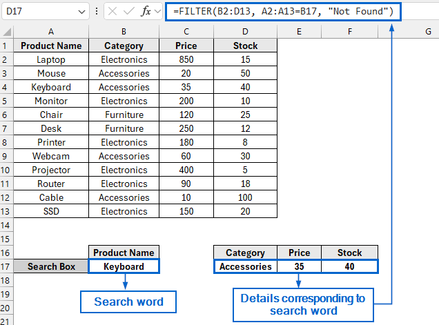
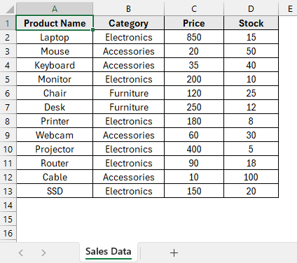
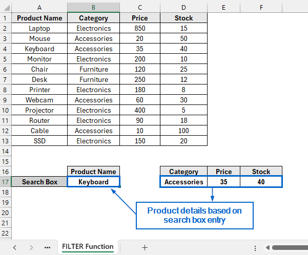
In the sample dataset, we have a worksheet called “Sales Data” containing information about Product Name, Category, Price and Stock. By using the FILTER function, we will create a search box that instantly returns full product details, Category, Price, and Stock whenever a Product Name is entered. We will display the modified dataset in a separate worksheet called “FILTER Function”.
The FILTER function in Excel is a powerful tool that extracts and displays only the rows from a dataset that meet specific, user-defined criteria. One disadvantage of this method is that it only works when there is an exact match between the search box entry and the dataset; it can not handle partial matches.
Steps:
➤ Open the FILTER Function worksheet, and in cell D17, put the following formula:
=FILTER(B2:D13, A2:A13=B17, "Not Found")
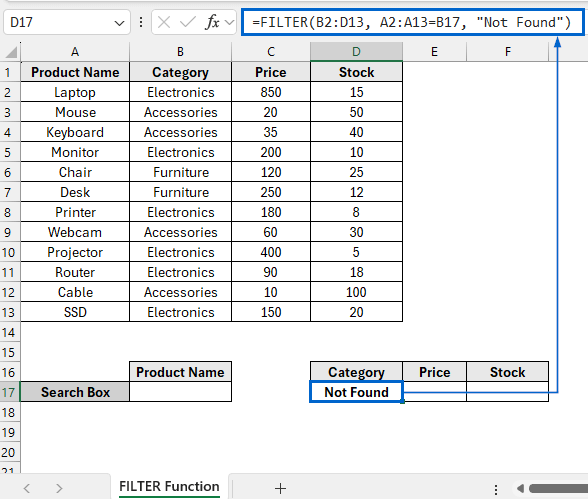
➧ B2:D13 is the range of data that we want to return results from.
➧ A2:A13=B17 is the condition that checks whether the values in column A (Product Name) match the value entered in cell B17 (Search Box).
➧ "Not Found" is the message displayed when no match is found.
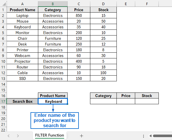
➤ Next, enter the name of the product that you want to search in cell B17.
➤ Cells D17, E17, and F17 should now display the Category, Price, and Stock details of the product, respectively, based on the search box entry.
Use FILTER with ISNUMBER Functions for Partial Matches
Both FILTER and ISNUMBER are powerful Excel functions that can be combined to create a dynamic search box. FILTER extracts the relevant rows from a dataset, while ISNUMBER checks whether the search keyword appears anywhere within the text, allowing for more flexible searches.
Unlike the previous method, this approach can handle partial searches, meaning it can return results even if only part of the search term matches with the dataset. Working with the same dataset, we will use the FILTER and ISNUMBER functions to create a search box and display the updated dataset in a separate worksheet called “FILTER with ISNUMBER Function”.
Steps:
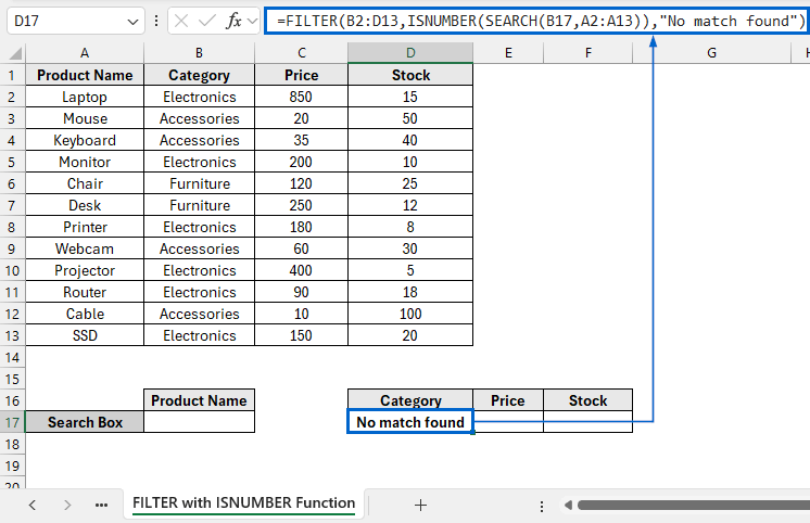
➤ Open the FILTER with ISNUMBER Function worksheet, and in cell D17, put the following formula:
=FILTER(B2:D13,ISNUMBER(SEARCH(B17,A2:A13)),"No match found")
➧ B2:D13 is the range of dataset from which results will be returned.
➧ SEARCH(B17, A2:A13) is the condition that checks each cell in range A2:A13 to see if it contains the text entered in B17, returning a number if a match is found.
➧ ISNUMBER(...) converts the search result into TRUE or FALSE. It returns TRUE if the search term exists in the cell, and FALSE otherwise.
➧ "No match found" is the message displayed if no matches are found.
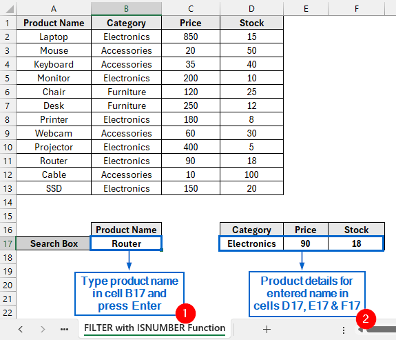
➤ Next, type the product name you want to search in cell B17 and press Enter.
➤ The complete details of the product, including category, price and stock, should now be displayed in cells D17, E17, and F17, respectively.
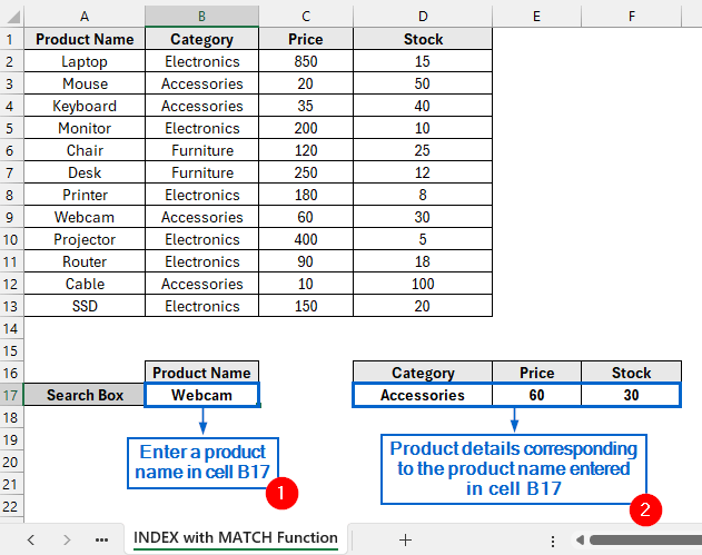
Use INDEX with MATCH for Individual Results
The MATCH function in Excel identifies the position of a search term within a dataset, while INDEX retrieves the corresponding value from a specified column. By combining these two functions, we can create a functional search box that displays results from the dataset.
This method allows users to return individual values for the entered data, as opposed to the previous methods, which display all details at once. Working again with the same dataset, we will now use INDEX with MATCH functions to create a search box. We will display the updated dataset in a separate “INDEX with MATCH Function” worksheet.
Steps:
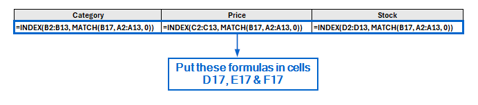
➤ Open the INDEX with MATCH Function worksheet, and in cell D17, put the following formula:
=INDEX(B2:B13, MATCH(B17, A2:A13, 0))
➧ MATCH(B17, A2:A13, 0) searches for the position of value entered in cell B17 within range A2;A13. The 0 at the end ensures an exact match.
➧ INDEX(B2:B13, …) uses the position provided by MATCH to retrieve the corresponding value from B2:B13.
➤ Again, in cells E17 and F17, enter the following formulas respectively:
=INDEX(C2:C13, MATCH(B17, A2:A13, 0))
=INDEX(D2:D13, MATCH(B17, A2:A13, 0))
Note:
The first formula is used to find the product price from column C, and the second formula retrieves the stock from column D.
➤ Now, when you type a product name in cell B17, the formula will return the corresponding value from the specified column.
Note:
You can control what the search box returns by entering a formula for each specific field.
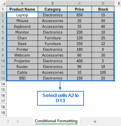
Highlight Search Results with Conditional Formatting
Excel’s Conditional Formatting is a useful tool that lets users visually change the appearance of cells based on defined rules or conditions. Unlike previous methods, creating a search box using Conditional Formatting will allow us to highlight the matching results directly within the dataset, including all related information in the row.
We will again work with the same dataset and create a fully functional search box using the Conditional Formatting tool. We will store the modified dataset in a separate “Conditional Formatting” worksheet.
Steps:
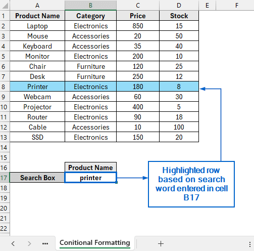
➤ Open the Conditional Formatting worksheet and highlight the range of cells A2 to D13.
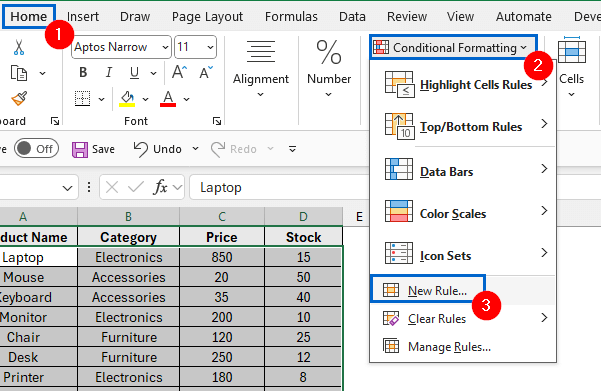
➤ Next, from the main menu, head to Home >> Conditional Formatting >> New Rule.
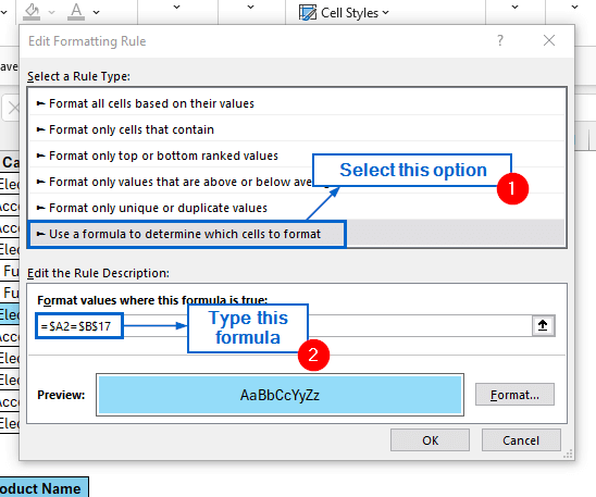
➤ Under Rule Type, select Use a formula to determine which cells to format and put the following formula:
=$A2=$B$17
Note:
This formula checks whether the value in column A (Product Name) of each row matches the search keyword entered in cell B17. If the condition is true, Excel will apply the chosen formatting and highlight the entire row.
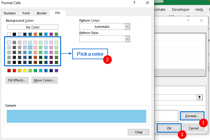
➤ Click Format, pick a Fill Color of your choice, and press OK to confirm the formatting.
➤ Now, when you type a search term in cell B17, the corresponding row in the dataset will be highlighted automatically.
Frequently Asked Questions
Can I Highlight Partial Matches Using Conditional Formatting?
Yes, you can easily highlight partial matches using Conditional Formatting by combining ISNUMBER with the SEARCH function. Head to Home >> Conditional Formatting and use the following formula:
=ISNUMBER(SEARCH($B$18, $A2))
What is the Best Approach When Working with Growing Datasets?
If your dataset grows larger, using the INDEX with MATCH function would be the most efficient approach for creating a search box.
The INDEX with MATCH method retrieves individual values directly from a dataset without returning the entire row at once, making the search box faster and more efficient as the dataset grows.
Concluding Words
Knowing how to create a search box in Excel is necessary for efficiently navigating large datasets, quickly locating specific information, and improving data analysis.
In this article, we have discussed four useful methods of creating a search box in Excel, including using the FILTER Function, FILTER with ISNUMBER Function, INDEX with MATCH Function and Conditional Formatting. Feel free to try out each method and choose one that best aligns with your needs.