Google Sheets has a smart feature that lets you automatically hide rows based on the value in a cell. The feature known as Filter View which is one of the easiest ways to keep your spreadsheets organized and easier to work with. This means you can quickly clean up your view and focus on what’s important.
This feature is especially helpful when you’re working with long lists or trying to isolate key information. In this guide, we’ll learn two most used methods to hide rows based on cell value using Filters in Google Sheets and Add Script. Also, we’ll guide you on how to create Filter Views, apply Filter by Condition, and add a simple Script to automate the process.
Suppose we want to hide specific rows in Column B that have values less than 1000. Here’s a step-by-step guide on how you can hide rows based on cell value in Google Sheets:
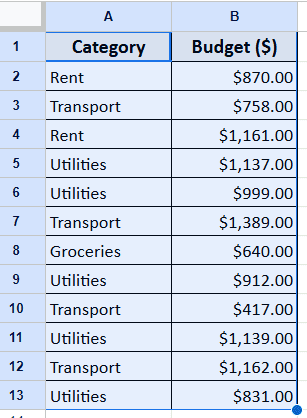
➤ Open your Google spreadsheet and select the range of cells or columns where you want to apply the Filter View. For Example, here we’re selecting the entire table, including Column A and Column B.
➤ Go to the Home tab and then click Data >> Create Filter View.
➤ Now your columns are activated for Filter View and you will see a filter icon next to each column header.
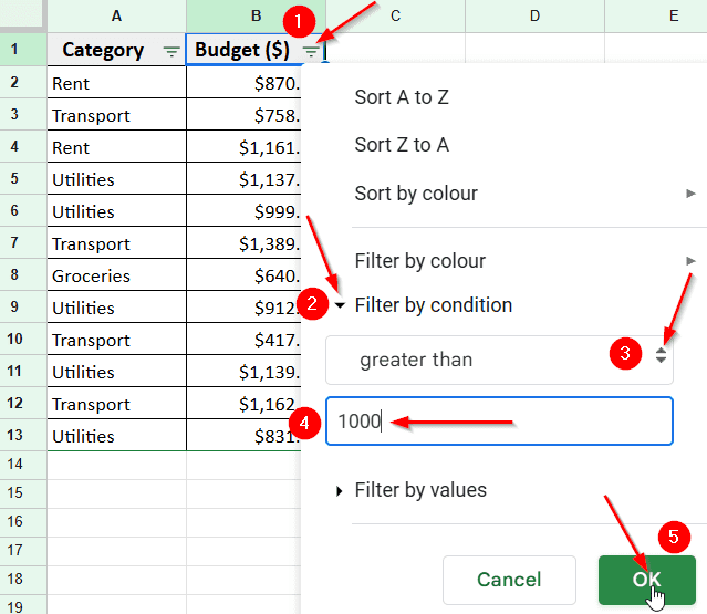
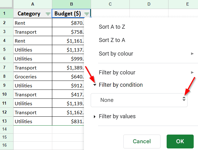
➤ Click the Filter Icon next to the column header “Budget ($)” in Column B and this will open the filtering options for that column.
➤ From the dropdown menu, select Filter by condition. This opens a set of rules you can apply to your data.
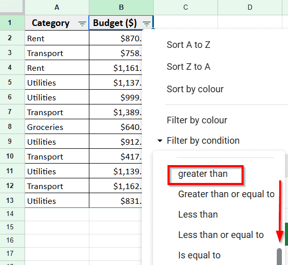
➤ Click on the dropdown under the condition section and choose the rule you want to use. Here we choose Greater than option.
➤ Type the value that you want to use as the filter. Since we want to hide rows that have values less than 1000 so we enter 1000.
➤ Click OK, and Google Sheets will instantly hide the rows that don’t match the condition you set.
Apply Filter to Hide Rows Based on Cell Value
This method involves two simple steps to hide rows in Google Sheets based on a specific cell value. First, you need to create a Filter View for the range you want to work with. Then, apply a Filter Condition to display only the rows that meet your criteria.
Step 1: Create Filter View In Google Sheets
Before hiding rows based on cell values in Google Sheets, you need to create a Filter View for the range of columns you want to filter. Because without creating a filter view you won’t be able to apply any filters.
Here is how you can do it:
➤ Highlight the columns you want to apply a filter to. For example, here we select an entire table of Column A and Column B.
➤ Go to the top Menu and click on Data, then choose Create filter view from the drop down menu.

➤ Now, you’ll see filter icons appear next to each column header. This means Filter View is active and ready for customization.
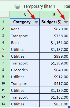
Once your filter view is set, it will be automatically saved and appear at the top-left of the sheet.
Step 2: Use Filter By Condition To Hide Rows
Suppose we want to hide specific rows in Column B that have values less than 1000. Here’s a step-by-step guide on how you can hide rows based on cell value in Google Sheets:
➤ Click the Filter Icon next to the column header “Budget ($)” in Column B and this will open the filtering options for that column.
➤ From the dropdown menu, select Filter by condition. This opens a set of rules you can apply to your data.
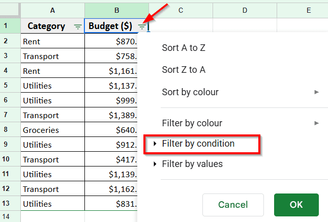
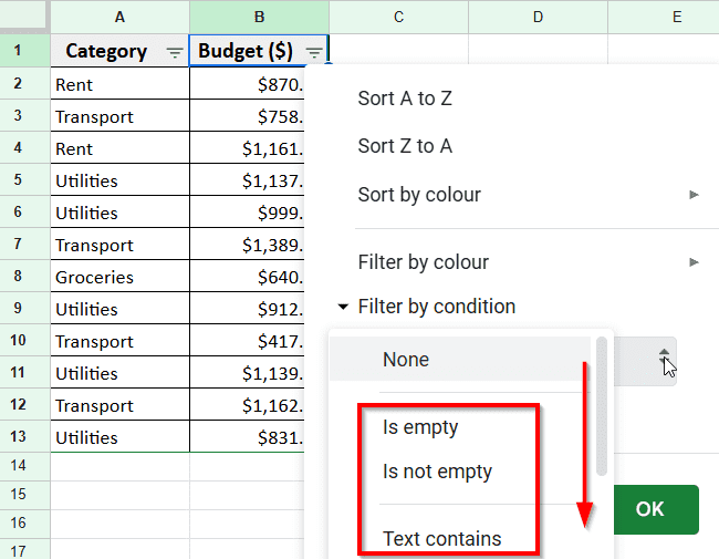
➤ Once you click Filter by condition, an empty box will appear where you can select any rules from the list.
➤ Scroll down and you will find the option you are looking for.
➤ Click on the dropdown under the condition section and choose the rule you want to use. Here we choose Greater than option from the list.
➤ Now, type the value that you want to use as the filter in the empty box below. For example, we put 1000.
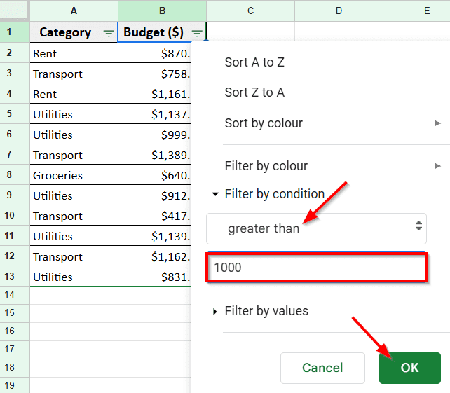
➤ Click OK, and Google Sheets will instantly hide the rows that don’t match the condition you set.
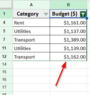
Only rows with values greater than 1000 will remain visible; the rest will be hidden from view.
Hide Rows Based on Cell Value Using Google Apps Script
If you want to automate the process, using Google Apps Script is a powerful option. This method involves writing a simple script that scans your data and hides rows based on the condition you set. For Example, here we want to hide all rows where the Paid checkbox is checked.
Here is how you can do it:
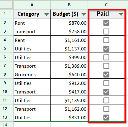
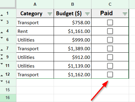
➤ In your table, Column C contains checkboxes to mark items as paid. Let’s create a script that hides any row where the checkbox is checked (TRUE).
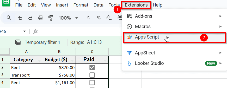
➤ Go to the Home tab and then click Extensions >> Apps Script
➤ Delete any default code and paste the Script above.
➤ Press the ▶️ Run button to execute the script. Follow the below image.
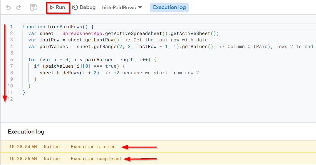
function hidePaidRows() {
  var sheet = SpreadsheetApp.getActiveSpreadsheet().getActiveSheet();
  var lastRow = sheet.getLastRow(); // Get the last row with data
  var paidValues = sheet.getRange(2, 3, lastRow - 1, 1).getValues(); // Column C (Paid), rows 2 to end
  for (var i = 0; i < paidValues.length; i++) {
    if (paidValues[i][0] === true) {
      sheet.hideRows(i + 2); // +2 because we start from row 2
    }
  }
}
➤ Accept authorization prompts the first time you run it.
➤ It will hide all rows where the checkbox in Column C is checked.
Add a Script to Unhide All Rows
If you want to restore the hidden rows later, you can use this helper script:
➤ Delete the previous code that you applied earlier and paste this reverse Script above.
➤ Press the Run ▶️ button to execute the script to reverse the effect and show all rows.
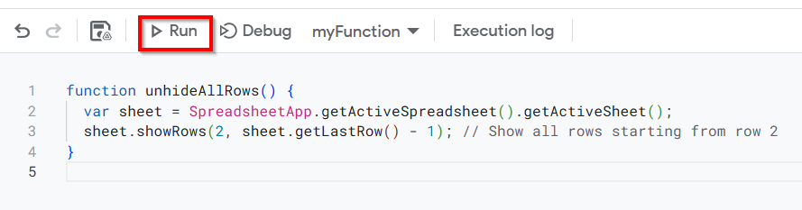
function unhideAllRows() {
  var sheet = SpreadsheetApp.getActiveSpreadsheet().getActiveSheet();
  sheet.showRows(2, sheet.getLastRow() - 1); // Show all rows starting from row 2
}
Frequently Asked Questions
How do you filter rows based on cell value in Google Sheets?
To filter rows based on a specific cell value, you have to create a Filter View first. Here’s how you can do it:
➤ Click on the filter icon in the column you want to filter
➤ Select Filter by condition, then choose a rule like Greater than or Text contains and enter your value.
➤ Google Sheets will instantly hide rows that don’t match the condition, without deleting any data.
Can you hide rows with conditional formatting?
No, conditional formatting only changes the appearance of cells like color or font style based on rules you set. It doesn’t actually hide rows. If you want to hide rows based on conditions, use the Filter View feature instead.
How do I automatically hide blank rows in Google Sheets?
To hide blank rows automatically:
➤ Apply a Filter View on the relevant column, then choose Filter by condition >> Is not empty.
➤ This will hide all rows where that column has a blank cell.
Wrapping Up
Filter View in Google Sheets is a simple but powerful feature that helps in hiding rows based on cell values. Instead of manually doing it, you can quickly filter out what you don’t need to see without changing the original data.
It’s perfect for reviewing specific values or collaborating on shared spreadsheets. Also, this feature reduces your workload and struggles with large datasets. You don’t need advanced skills to use it, and you’re in control of what’s visible.