Finding duplicate entries in Google Sheets is essential when working with lists like employee IDs, emails, or product codes to maintain data accuracy. Duplicates can cause errors or confusion, so spotting them quickly is key. The VLOOKUP function is a straightforward way to identify if a value appears more than once within the same dataset.
In this article, you’ll explore different techniques to use VLOOKUP for finding duplicates within a single sheet. Whether you want to flag repeated values, mark duplicate rows, or extract lists of duplicates, we’ll guide you through step-by-step examples.
Steps to identify duplicate entries using VLOOKUP and ISNA functions in Google Sheets
➤ Stay on your working sheet with the employee list.
➤ Add a new column (e.g., Column D) and label it Duplicate Check.
➤ In cell D2, enter this formula:
=IF(ISNA(VLOOKUP(A2, A3:A, 1, FALSE)), “”, “Duplicate”)
➤ Press Enter and drag the formula down to check all rows.

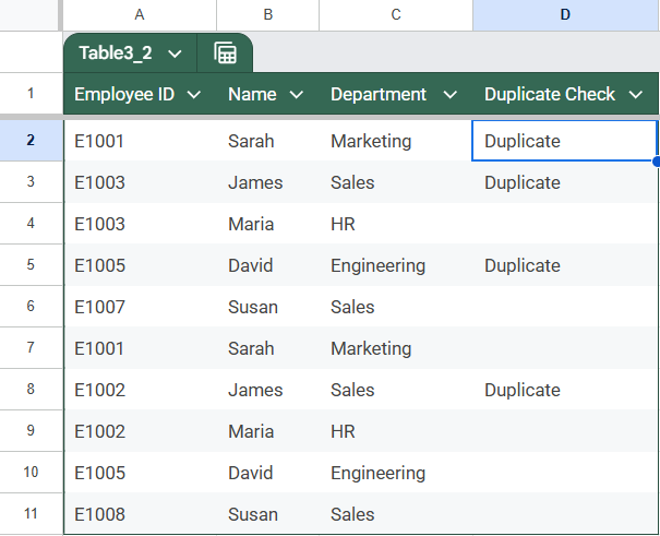
Identify Duplicate Entries Using VLOOKUP and ISNA Functions
This method uses the VLOOKUP and ISNA functions together to flag duplicate entries by checking if an Employee ID appears more than once within the same sheet. Specifically, it compares each ID against the entire Employee ID column to identify repeated values.
The VLOOKUP function looks for the current Employee ID further down the list, and ISNA checks whether a duplicate match was found. If a match is found, the formula flags it as a duplicate, helping you quickly spot repeated records in your dataset.
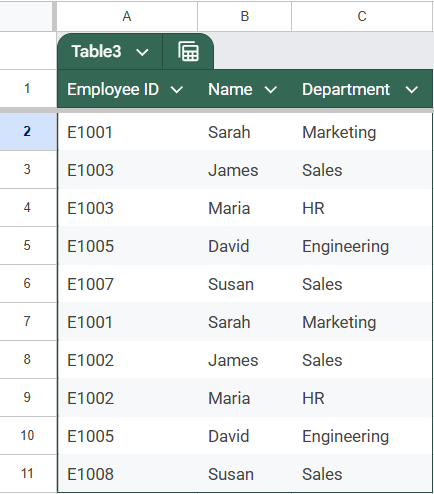
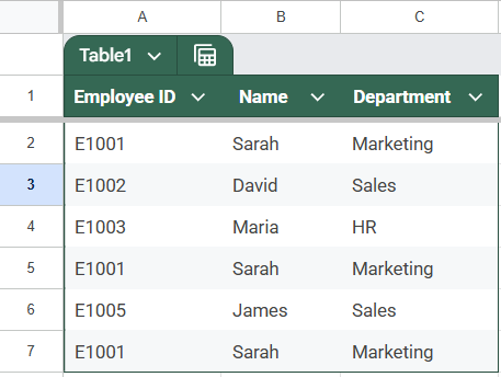
This is the dataset we will be using for this article:
Steps:
➤ Stay on your working sheet with the employee list.
➤ Add a new column (e.g., Column D) and label it Duplicate Check.
➤ In cell D2, enter the following formula:
=IF(ISNA(VLOOKUP(A2, A3:A11, 1, FALSE)), “”, “Duplicate”)
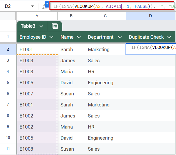
➧ A3:A is the range below the current row in the same column where duplicates might appear.
➧ VLOOKUP searches for the current ID further down the list.
➧ If no duplicate is found, VLOOKUP returns an error.
➧ ISNA detects that error.
➧ IF returns "Duplicate" if a duplicate is found; otherwise, it leaves the cell blank.
➤ Press Enter and drag the formula down to check all rows.
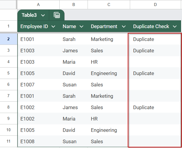
The first instance of each duplicate will be highlighted in Column E.
Flag Duplicate Entries Cleanly Using IFERROR with VLOOKUP Function
This approach wraps VLOOKUP inside IFERROR to flag duplicates without showing error messages. It compares each Employee ID against the rest of the column, highlighting duplicates while keeping your sheet tidy by hiding errors.
Instead of showing #N/A for unique entries, IFERROR replaces errors with a blank cell. The result displays “Duplicate” next to every repeated Employee ID found later in the list.
Steps:
➤ On your working sheet, add a column titled Check Status (e.g., Column E).
➤ In cell D2, enter this formula:
=IFERROR(IF(VLOOKUP(A2, A3:A, 1, FALSE)=A2, “Duplicate”, “”), “”)
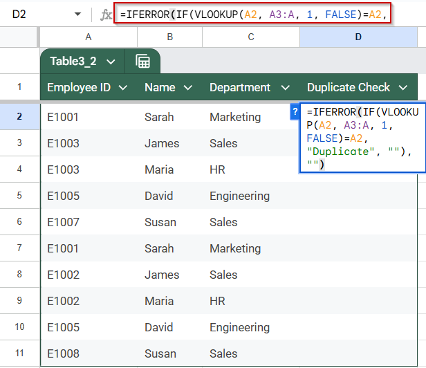
➧ A3:A is the range below the current row to search for duplicates.
➧ VLOOKUP looks for the current ID in the range.
➧ If a duplicate is found, it returns the ID, and the formula returns "Duplicate".
➧ If not, VLOOKUP throws an error.
➧ IFERROR handles the error and leaves the cell blank.
➤ Drag the formula down to apply it to all entries.
Use Helper Column & VLOOKUP Function to Find the Nth Duplicate
This method helps you identify the nth occurrence of duplicate values in a list using a helper column and VLOOKUP. It’s useful when you want to track how many times a particular entry appears and retrieve duplicates based on their occurrence order.
We have updated the dataset for this method:
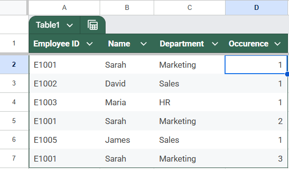
As you can see the Employee with ID E1001 has 3 entries on this sheet. A clear indicator of which duplicate each entry is (1st, 2nd, 3rd, etc.) and a way to extract specific duplicates using VLOOKUP.
Steps:
➤ Add a helper column next to your dataset in Sheet1, for example, Column D, and label it “Occurrence”.
➤ In cell D2, enter this formula to count the occurrence of each Employee ID up to that row:
=COUNTIF($A$2:A2, A2)
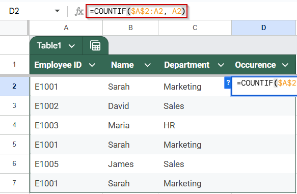
➤ Drag this formula down for all rows. This will number duplicates incrementally (1 for first occurrence, 2 for second, etc.).
➤ Now, to find the nth duplicate, use this VLOOKUP formula in cell E2. For example, to find the 2nd occurrence of an Employee ID from Sheet1:
=VLOOKUP(“E1001″&2, ARRAYFORMULA(A2:A7 & D2:D7), 1, FALSE)

➧ ARRAYFORMULA(A2:A & D2:D) combines the Employee ID and its occurrence number into a single string for lookup.
➧ The VLOOKUP searches for the Employee ID concatenated with the desired occurrence number (e.g., "E1001"&2 for the second occurrence).
➧ This returns the exact nth duplicate, allowing you to isolate duplicates by their occurrence order.
➤ Press Enter and drag the fill handle down.
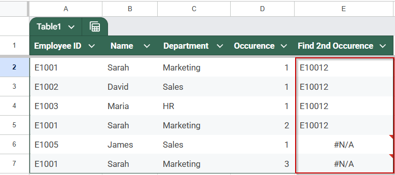
The formula will keep repeating the Employee ID mixed with the occurrence number until it has reached the second occurrence of the employee ID on the sheet, e.g, E10012. The 2 in the end is the occurrence number. After the nth occurrence the formula will return an #N/A error, letting you know that the nth occurrence has been detected.
Using this method, you can systematically identify and extract specific duplicates, which is useful for detailed data audits or reports.
Applying ARRAYFORMULA with VLOOKUP Function Across Entire Columns
This method uses the power of ARRAYFORMULA combined with VLOOKUP to check an entire column at once, flagging which entries in your first list also appear in the second list. Instead of dragging formulas row-by-row, this dynamic approach applies the formula across all rows automatically.
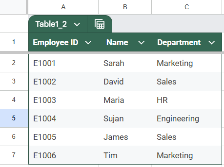
These are the datasets we will be using to demonstrate the next two methods. We have split our previous dataset and have moved them to two different sheets.
Sheet1 (Employee Information):
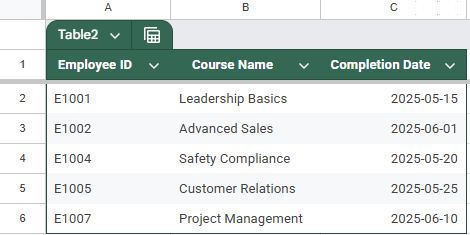
Sheet 2 (Course Information):
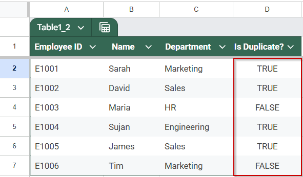
A new column that shows TRUE if an Employee ID in Sheet1 is found in Sheet2, or FALSE if it isn’t, all generated in one step without manual copying.
Steps:
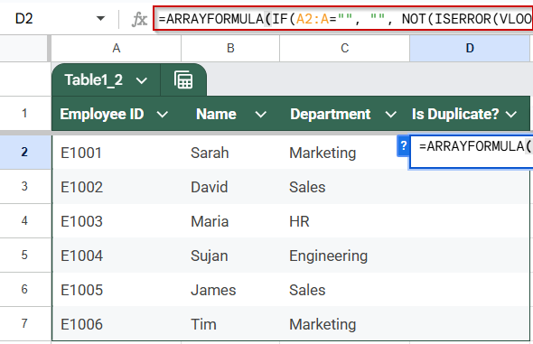
➤ In Sheet1, add a new column header, for example, Is Duplicate?.
➤ In cell D2, enter this formula:
=ARRAYFORMULA(IF(A2:A=””, “”, NOT(ISERROR(VLOOKUP(A2:A, Sheet2!A$2:A$6, 1, FALSE)))))
➧ VLOOKUP(A2:A, Sheet2!A$2:A$6, 1, FALSE) tries to find each ID from Sheet1 in the range on Sheet2.
➧ If VLOOKUP finds the ID, it returns a value; if not, it returns an error.
➧ ISERROR checks whether there was an error (no match).
➧ NOT(ISERROR(...)) flips TRUE/FALSE, so it’s TRUE when a match exists (duplicate).
➧ The outer IF ensures blank rows stay blank instead of showing TRUE or FALSE.
➤ Press Enter.
This formula automatically fills down as many rows as there are in column A, saving you from copying the formula manually and instantly highlighting duplicates across your datasets.
Extract Only Duplicate Values from One Column
This method helps you pull out just the duplicate values from one list by checking if those values also appear in another list. Using VLOOKUP combined with IFERROR and FILTER, it creates a clean list of duplicates without showing errors or blanks.
A filtered list showing only the Employee IDs from Sheet1 that also exist in Sheet2, perfect for focused analysis or reporting.
Steps:
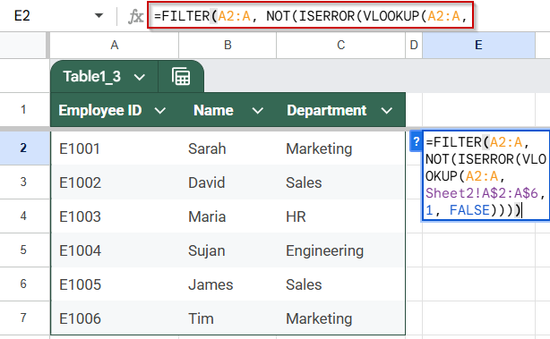
➤ In a new sheet or next to your data, choose a cell where you want the duplicate list to appear, say E2.
➤ Enter this formula:
=FILTER(A2:A, NOT(ISERROR(VLOOKUP(A2:A, Sheet2!A$2:A$6, 1, FALSE))))
➧ VLOOKUP(A2:A, Sheet2!A$2:A$6, 1, FALSE) searches for each ID from Sheet1 in the Employee ID column of Sheet2.
➧ If a match is found, VLOOKUP returns the value; if not, it returns an error.
➧ ISERROR(...) identifies which values did not match (errors).
➧ NOT(ISERROR(...)) returns TRUE for duplicates (found values).
➧ FILTER uses the TRUE/FALSE array to return only the duplicates from Sheet1’s list.
➤ Press Enter.
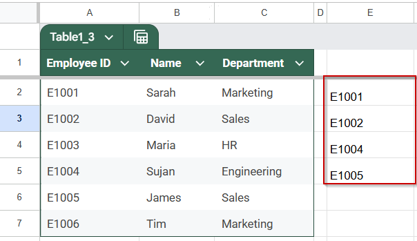
This method gives you a clean, compact list of duplicates for easy review or further processing, without cluttering your sheet with errors or empty rows.
Frequently Asked Questions
Can I use VLOOKUP to find duplicates within the same column in Google Sheets?
Yes! By adjusting the lookup range to start from the row below the current entry, VLOOKUP can check for repeated values within the same column. Combining it with functions like ISNA or IFERROR helps you flag duplicates without showing errors.
How does the helper column with COUNTIF help identify the nth duplicate?
The helper column uses COUNTIF to count how many times each value has appeared up to the current row, numbering each duplicate sequentially (1st, 2nd, 3rd, etc.). You can then use VLOOKUP with this occurrence number to find specific duplicates based on their order.
What advantages does using ARRAYFORMULA with VLOOKUP offer?
ARRAYFORMULA lets you apply a formula to an entire column at once, eliminating the need to drag formulas down manually. When combined with VLOOKUP, it can instantly flag duplicates across large datasets, saving time and reducing errors.
How can I extract a clean list of duplicates without showing errors or blanks?
You can use the FILTER function alongside VLOOKUP and ISERROR to create a filtered list that only shows duplicate values. This method avoids cluttering your sheet with error messages or empty rows, making it easier to review or analyze duplicates.
Wrapping Up
Managing duplicates in Google Sheets is essential for accurate data handling. By using VLOOKUP with functions like ISNA, IFERROR, COUNTIF, and ARRAYFORMULA, you can quickly identify and flag duplicates both within a single sheet and across multiple sheets. Helper columns and filtered lists provide additional ways to analyze duplicate occurrences effectively. Applying these techniques helps maintain clean data, avoid errors, and improve reporting accuracy. Try these methods to streamline your workflow and keep your data organized effortlessly.