Splitting cells in Google Sheets is a very useful skill for certain types of jobs. For example, you exported data from a CRM or PDF, and now you want to split names, product codes, etc.
In that case, you have to split cells horizontally. Sadly, Google Sheets doesn’t give you those options by default.
But we have solutions for that. In this article, we will talk about 5 different techniques to split cells horizontally in Google Sheets for different use cases. Let’s dive in.
➤ Click the cell you want to split
➤ Go to Data > Split text to columns
➤ Choose the delimiter (comma, space, etc.) In this case, choose space.
➤ You will instantly see your data in different horizontal cells.
Use the 'Split Text to Columns' Feature (Menu Option)
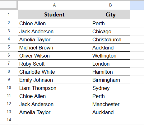
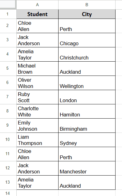
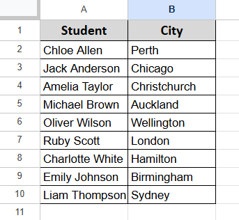
In the following dataset, we have a list of students in Column A and their cities in Column B.
What we will do here is split the name cells into two columns. One will contain the first name and the other the last name.
We’re going to do this in the dataset using Google Sheets’ built-in Split Text to columns feature.

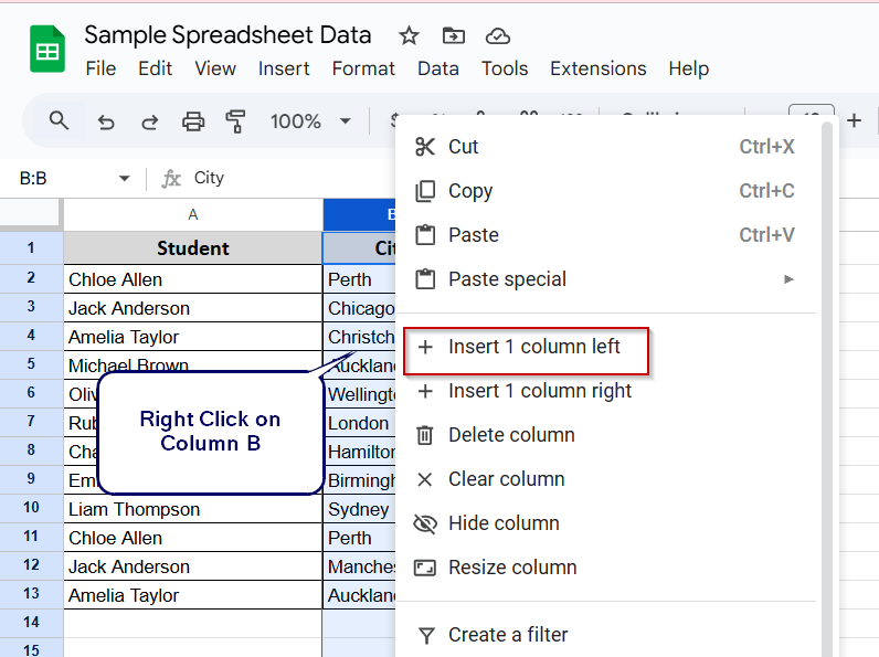
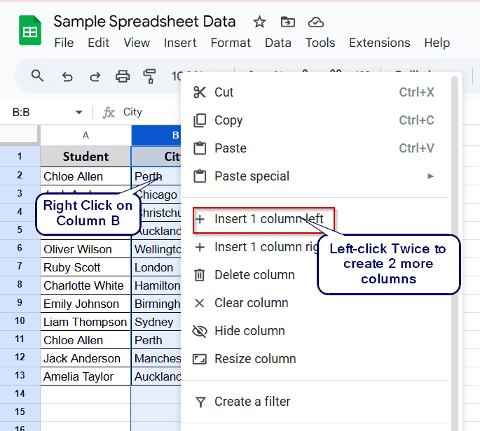
➤ First, we have to insert a new column to protect the City data.
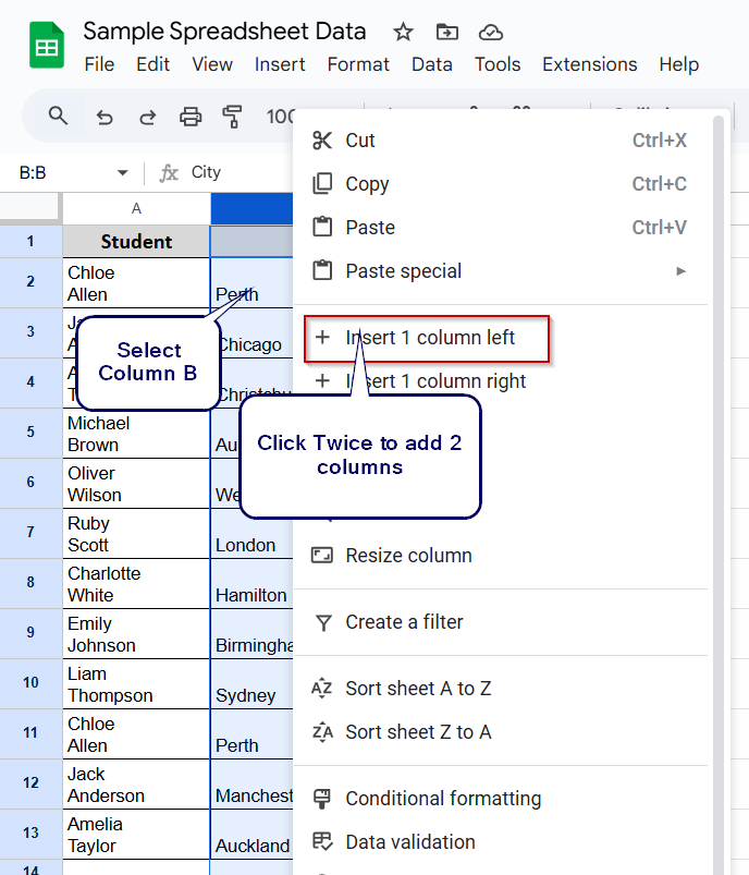
➤ Right-click on Column B (the City column) and choose Insert 1 column left. This will push your city data into Column C. If we don’t do this, we will lose our city data.
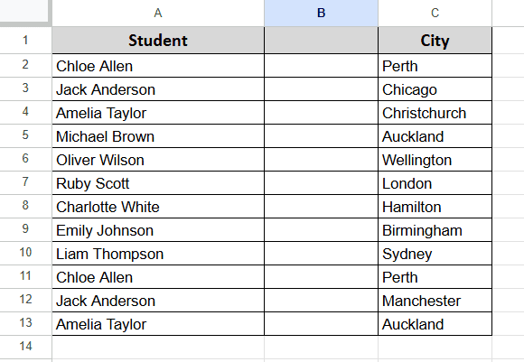
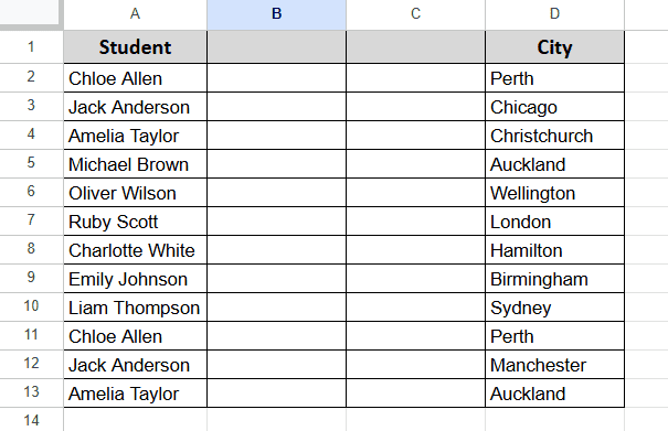
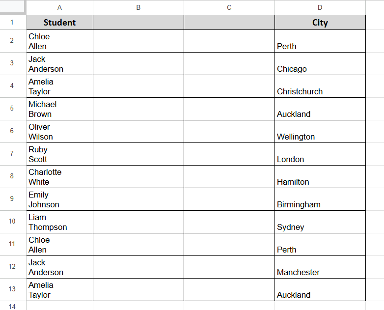
➤ Now our datasheet will look like this.
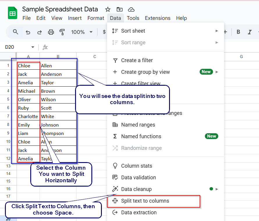
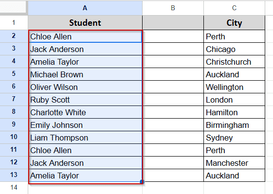
➤ Select the entire Student Name column (Column A).
➤ Go to the Data menu from the top of the worksheet and select Split Text to Columns from the drop-down menu.
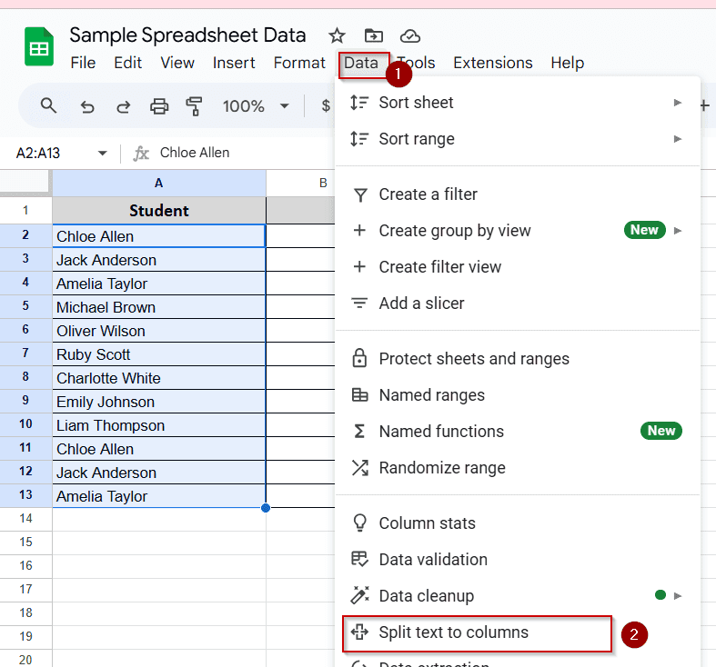
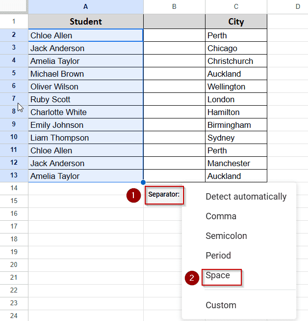
➤ A small pop-up will appear. It will show “Separator: Detect Automatically.” When you click, you will see multiple options, as shown in the screenshot below. You can select according to your worksheet type. In this case, we will select space.
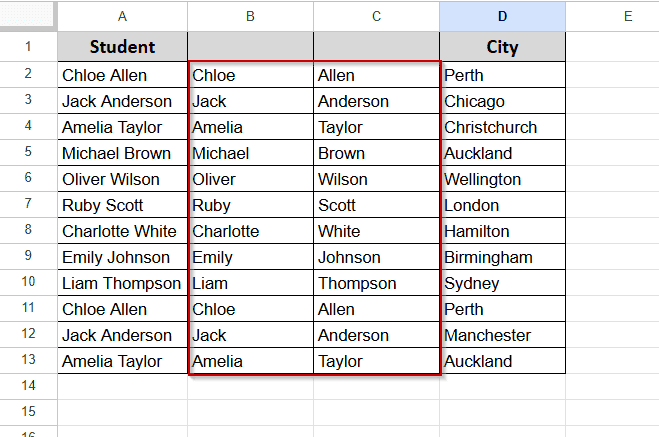
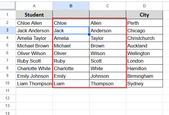
➤ That’s it. Now you will see First Name in Column A, Last Name in Column B, City remains safe in Column C.
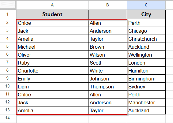
Finally, you can change the column header if you make the dataset more readable.
Note:
If you don’t make the extra column, you will lose the data inside the column. So, be careful before you practice this on any important sheet.
Use the SPLIT Function for Dynamic Data Formatting
This method is helpful when you want more control over your data. It will split your data into two new columns. Let’s see how to do that.
Unlike the manual “Split text to columns” method, this one is formula-based. Therefore, data will be automatically updated.
We are going to use the previous dataset. You can see the screenshot below:
➤ First, insert two new columns between the Student Name column and the City column. It will keep your city column data safe. Here is how you will do it.
➤ Now your dataset will have 2 extra columns. Your city data will be in Column D.
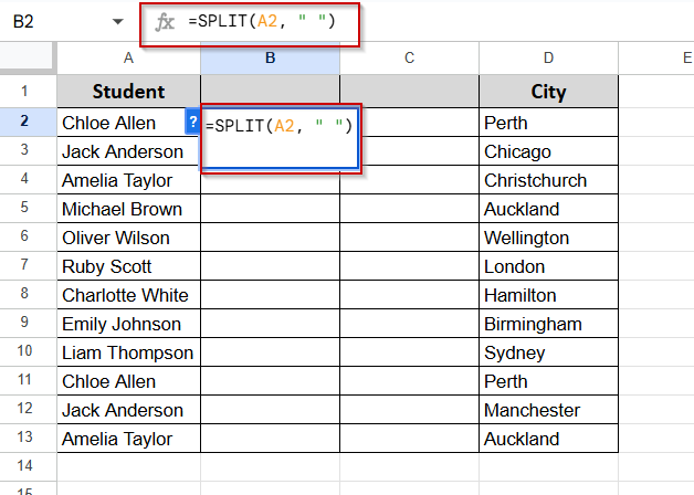
➤ Now double click on B2 and write the formula: =SPLIT(A2, ” “) and hit Enter.
➤ You will see that your data is in Column B and Column C.
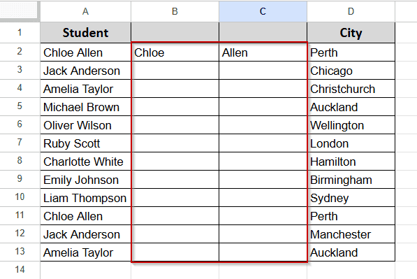
➤ Now drag the fill handle down as long as your data goes. And you will see your data like the screenshot below:
Note:
The main benefit of this method whenever you change any data on the Student Column, it will automatically update the next two columns.
REMINDER: Don’t forget to create 2 extra columns first before applying this method to secure your city data.
SPLIT Cell Horizontally by Line Breaks
In the following dataset, we have a list of students in Column A and their cities in Column B. But this time, you will see that each cell in Column A contains a line break between the first and last name.
This often happens if someone enters names manually using Alt + Enter or pastes in from Word or PDFs.
In this case, our previous methods won’t work. Therefore, we will use the SPLIT by Line breaks method.
Let’s do it then.
➤ First, insert two empty columns between the Student column and the City column, like the previous method. It will save your city data.
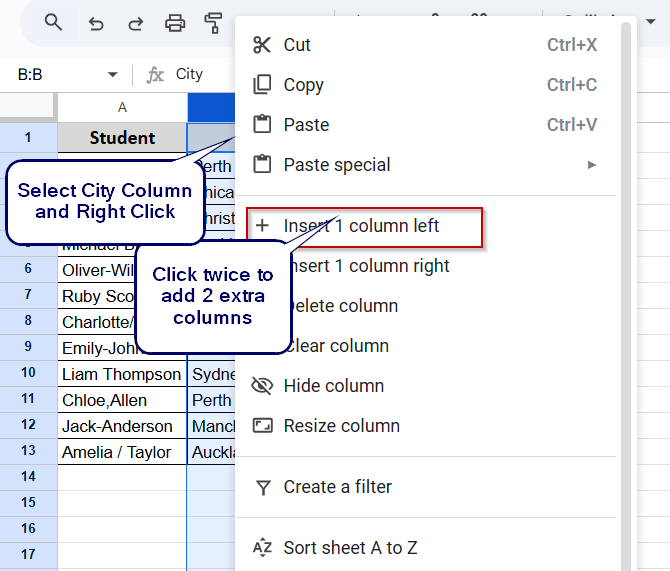
➤ To do that, right-click on your City data and click on Insert One-Column Left and do that twice.
➤ Your dataset will look like the screenshot below now.
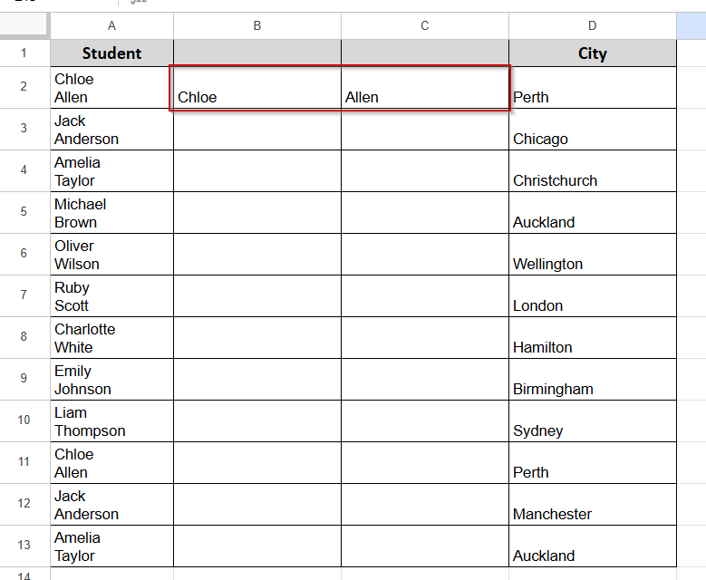
➤ Now, click on cell B2 and Write this formula =SPLIT(A2, CHAR(10)) and hit Enter.
➤ You will see the first name appear in B2, and the last name in C2.
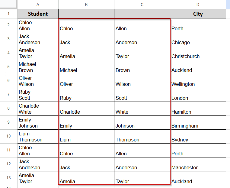
➤ Now drag the formula down to apply it to the entire column.
Note:
This method is handy when the Data on your Google Sheets is broken by line breaks.
Use the REGEXEXTRACT Function
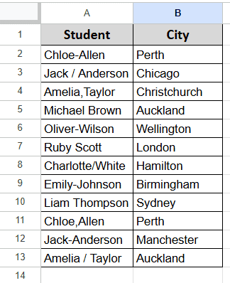
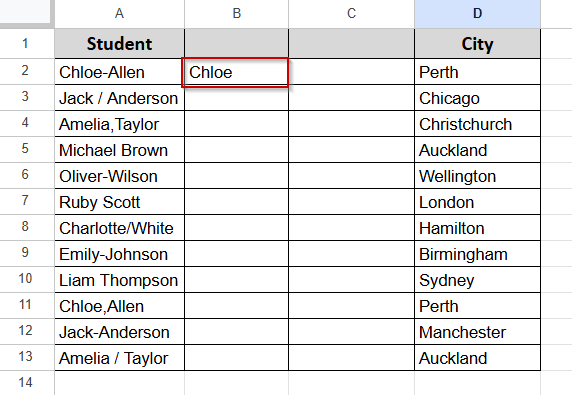
In the following dataset, we have student names in Column A and their cities in Column B.
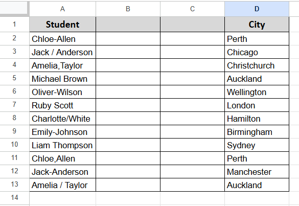
But this time, the formatting of the name section is not consistent. Some use dashes, some use slashes, others use commas or even multiple spaces. We can see entries like these:
Jack – Anderson, Amelia,Taylor, Michael Brown, and Emily-Johnson.
In these types of scenarios, the SPLIT function can not handle the data. Therefore, we need to apply the REGEXEXTRACT function, which will help you to break the pattern.
➤ First, insert two empty columns between the Student column and the City column, like the previous method. It will save your city data.

➤ Now you will see your dataset like the screenshot below:

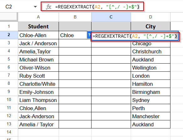
➤ Click on cell B2 and write the formula =REGEXEXTRACT(A2, “^[^,/ -]+”) and hit enter.
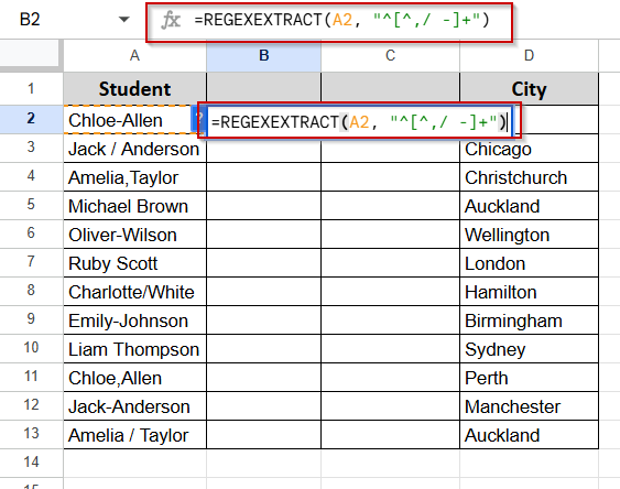
➤ It will extract the first name.
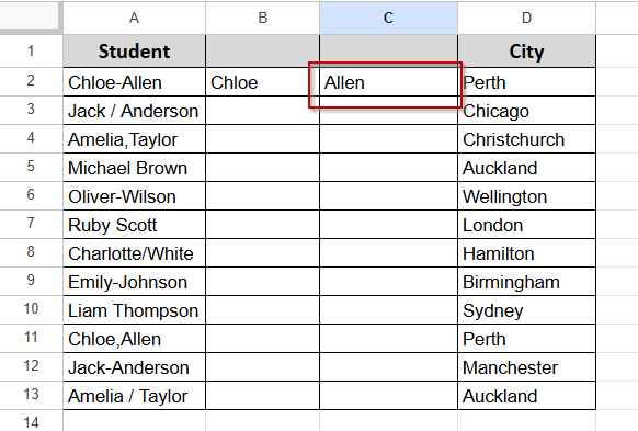
➤ Now apply the same formula =REGEXEXTRACT(A2, “[^,/ -]+$”) in the next cell C2.
➤ It will extract the second name.
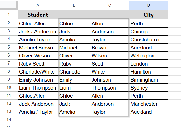
➤ Now, just drag both formulas down to apply them to all rows.
Note:
This method is handy when your data is not formatted properly.
SPLIT + ARRAYFORMULA to Handle Multiple Rows at Once
We will use one of our previous worksheets here. But first, let us explain to you the purpose of this method. Let’s say you are dealing with lots of data, like 500 or 5000, in a column. In that case, using the SPLIT formula and dragging data is quite a hassle.
But if you use SPLIT + ARRAYFORMULA, it will automatically fill all the cells. Fantastic, isn’t it? Let’s do it then. Here is our dataset.
➤ First, insert two empty columns between the Student column and the City column, like the previous method. It will save your city data.
➤ Now your dataset will have 2 extra columns. Your city data will be in Column D.
➤ In cell B2 enter this formula: =ARRAYFORMULA(IF(A2:A=””, “”, SPLIT(A2:A, ” “))) and hit Enter.
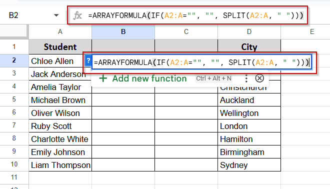
➤ You will see all the cells are filled with first and last names, and no need to drag to complete the task.
Note:
This method will only work if all of your data is separated with a space and there are no formatting issues in your original data. If your cells have line breaks, slashes, or extra spaces, use other methods like REGEXEXTRACT or SPLIT by line breaks.
Frequently Asked Questions
Can I split a cell using multiple delimiters, like commas and hyphens?
Yes, you can do that by using the REGEXEXTRACT Function that we showed in this tutorial.
What should I do if the Split Text to columns feature overwrites existing data?
It happens if you don’t create extra columns before splitting the data. So, always create an extra column to give space for the split data. And don’t forget to have a backup before applying any split method to make sure your original data is safe.
Are there add-ons that can help with splitting cells?
Yes. There are several add-ons. You can search online and find one that suits your needs.
Can I automate splitting cells using Google Apps Script?
Yes. Google Apps Script gives you the option to write custom functions to split data automatically.
Concluding Words
In this article, you learned how to split a cell horizontally in Google Sheets. We showed different techniques. You can use the first option, which is using the Split Text to Columns from the Data menu for the simple dataset.
On the other hand, for a huge dataset, you can use SPLIT + ARRAYFORMULA.
We have attached all the worksheets used in this article.
Download our practice workbook for practicing. Also, you can ask any questions in the comment section below, and we would be more than happy to help you.