The QUERY function in Google Sheets is a powerful tool for summarizing and analyzing data, especially when you need to group values across more than one column. Whether you’re managing sales reports, attendance logs, or inventory data, grouping by multiple columns helps you break down trends and comparisons by multiple dimensions, like category and region, or date and product.
In this article, you’ll learn how to use the GROUP BY clause inside the QUERY function to combine and summarize rows based on two or more columns. We’ll walk through practical examples to help you organize your dataset efficiently without using pivot tables or manual sorting.
Steps to group data by multiple columns in Google Sheets using the QUERY function:
➤ Use a dataset in A1:E11 with columns: Date, Region, Product, Units Sold, and Revenue.
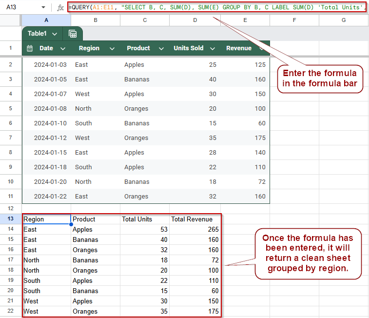
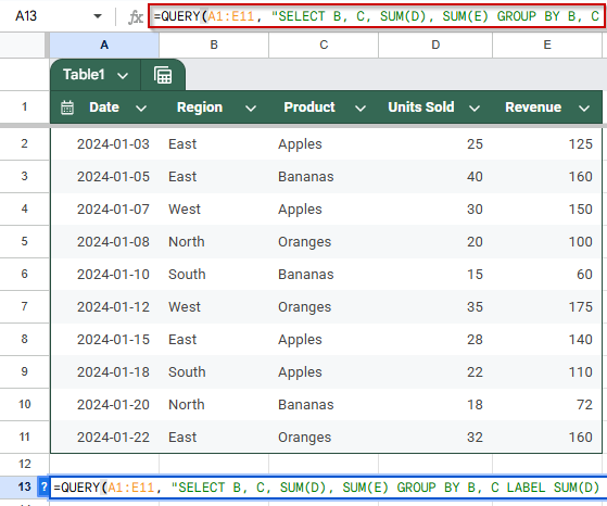
➤ In cell A13, enter the formula:
=QUERY(A1:E11, “SELECT B, C, SUM(D), SUM(E) GROUP BY B, C LABEL SUM(D) ‘Total Units’, SUM(E) ‘Total Revenue'”, 1)
➤ Press Enter.
Use QUERY to Group by Multiple Columns in Google Sheets
The QUERY function in Google Sheets lets you group data based on multiple columns using the GROUP BY clause. This is especially useful when you want to summarize totals, averages, or counts across combinations like Region and Product. Instead of manually sorting or creating pivot tables, this method lets you write one formula to generate grouped summaries directly in your sheet.
Steps:
➤ Use the sample dataset in cells A1:E11, which contains Date, Region, Product, Units Sold, and Revenue.
➤ To group the data by Region and Product and calculate total Units Sold and Revenue, enter the following formula in cell A13:
=QUERY(A1:E11, “SELECT B, C, SUM(D), SUM(E) GROUP BY B, C LABEL SUM(D) ‘Total Units’, SUM(E) ‘Total Revenue'”, 1)
➧ GROUP BY B, C: Groups the result by Region and Product.
➧ LABEL …: Renames the columns for a more readable output.
➧ 1: Tells the QUERY function that row 1 contains headers.
➤ Once you press Enter, Google Sheets will display a neatly grouped table showing total units and revenue for each product within each region.
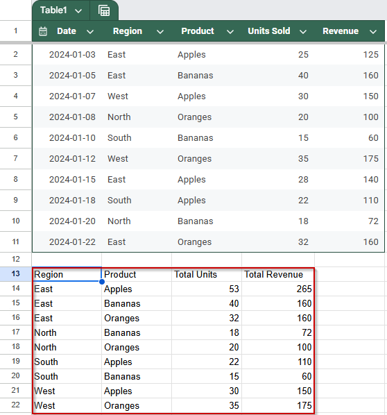
➤ This method is ideal when you want to generate summary reports across two dimensions, such as total sales by region and product type, all with one formula.
Combine GROUP BY with WHERE Clause for Filtered Grouping
When working with large datasets, you might want to group data across multiple columns but only for a specific condition, like a particular region or time period. By combining the GROUP BY clause with a WHERE condition in the QUERY function, you can target and summarize only the data that matters to you. This approach is helpful for generating segmented reports, such as sales totals for one region or specific products.
Steps:
➤ Start with the dataset in cells A1:E11, which includes Date, Region, Product, Units Sold, and Revenue.
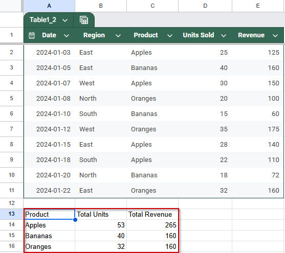
➤ To show only totals for the “East” region grouped by Product, enter this formula in cell A13:
=QUERY(A1:E11, “SELECT C, SUM(D), SUM(E) WHERE B = ‘East’ GROUP BY C LABEL SUM(D) ‘Total Units’, SUM(E) ‘Total Revenue'”, 1)
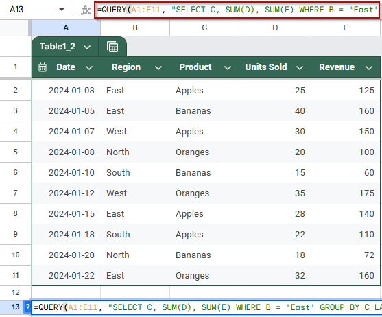
➧ WHERE B = 'East': Filters the data to include only rows where Region is East.
➧ GROUP BY C: Groups the remaining rows by Product.
➧ LABEL …: Adds readable column labels.
➧ 1: Indicates the presence of headers in row 1.
➤ After pressing Enter, the table will display only the products sold in the East region, along with their total units and total revenue. This focused summary helps quickly analyze performance in that specific region
➤ This method is best when you want to analyze subsets of your data, like comparing sales performance for one region or department, while still summarizing by multiple criteria.
Group by Multiple Columns and Sort Results
You can combine the GROUP BY clause with ORDER BY in the QUERY function to both aggregate your data and sort the grouped results according to your preferences. This technique is helpful when you want to summarize information across multiple categories and then order those summaries meaningfully, such as sorting sales totals by region and product.
Steps:
➤ Use the dataset in cells A1:E11 containing Date, Region, Product, Units Sold, and Revenue.
➤ To group sales data by Region and Product, then sort the results by Region ascending and total Revenue descending, enter this formula in cell A13:
=QUERY(A1:E11, “SELECT B, C, SUM(D), SUM(E) GROUP BY B, C ORDER BY B ASC, SUM(E) DESC LABEL SUM(D) ‘Total Units’, SUM(E) ‘Total Revenue'”, 1)
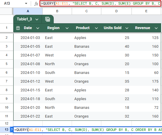
➧ GROUP BY B, C: Groups data by both Region and Product.
➧ ORDER BY B ASC, SUM(E) DESC: Sorts groups first by Region (A to Z), then by total Revenue (highest to lowest).
➧ LABEL: Adds user-friendly column headers for totals.
➧ 1: Indicates the first row contains headers.
➤ After pressing Enter, the table displays grouped sales data sorted to highlight the highest-earning products within each region.
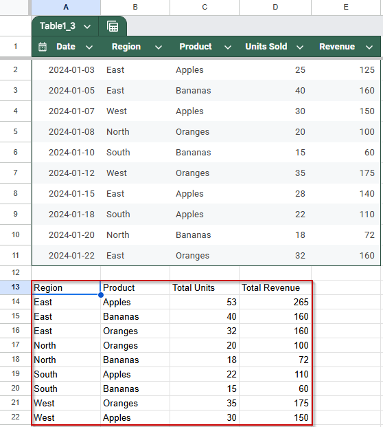
This method allows you to create clear, organized summaries that combine multiple grouping criteria with custom sorting to analyze your data effectively.
Frequently Asked Questions
Can I group by more than two columns using the QUERY function?
Yes, you can group by as many columns as needed by listing them in the GROUP BY clause. For example, GROUP BY B, C, D will group by three columns. Just ensure that any column in the SELECT statement that isn’t aggregated (like SUM, AVG) is included in GROUP BY.
What happens if I don’t use the LABEL clause in my QUERY?
If you omit the LABEL clause, Google Sheets will assign generic labels like sum D or sum E to your aggregated columns. The formula will still work, but using LABEL improves readability and makes your report easier to understand.
Can I apply filters before grouping data?
Absolutely. You can use a WHERE clause before GROUP BY to filter your data. For example, to group only for the “East” region, use: WHERE B = ‘East’ GROUP BY C
How is this different from using a pivot table in Google Sheets?
While pivot tables offer a drag-and-drop interface, the QUERY function gives you a formula-based approach that’s more dynamic and flexible, especially when you need to automate or replicate summaries across different sheets or dashboards.
Wrapping Up
Using the QUERY function to group by multiple columns in Google Sheets is a powerful way to summarize and analyze data without relying on manual sorting or pivot tables. Whether you’re aggregating sales by region and product or tracking metrics across categories, this method keeps your reports dynamic, clean, and easily adjustable. With just one formula, you can create clear, data-driven summaries that scale with your dataset.