Need to total numbers only when a related cell contains certain text? Google Sheets makes this easy with the SUMIF function. Whether you’re adding up sales by region or expenses by keyword, SUMIF helps you get the right totals without manual filtering.
In this article, we’ll walk through simple ways to use SUMIF when a cell contains specific text, including exact matches and partial phrases, using a sample dataset of regional sales.
Steps to sum values based on an exact text match:
➤ Use case: Total sales where a specific condition (e.g., Region = “East”) is met.
➤ Dataset example: Column B contains region names, Column C contains sales amounts.
➤ Click on the result cell (e.g., E2) in your Google Sheet.
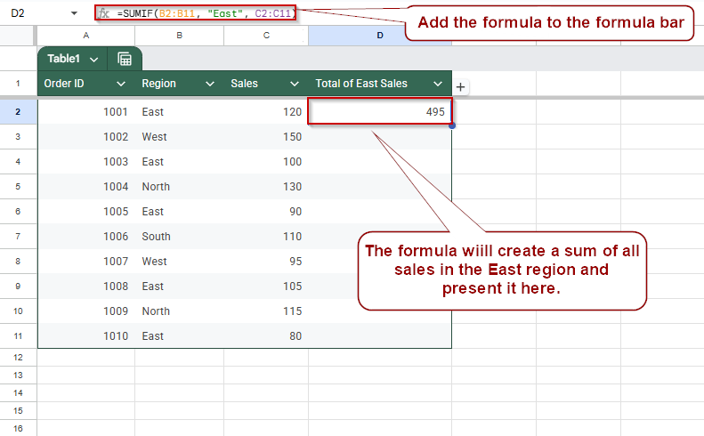
➤ Enter the formula: =SUMIF(B2:B11, “East”, C2:C11)
➤ Press Enter to display the result.
Sum Values When a Cell Matches Exact Text Using SUMIF in Google Sheets
When you want to total values in one column only if a related column contains an exact match (like summing sales for a specific region), SUMIF is the go-to function. This method is ideal for simple conditional totals where the criteria are clearly defined, such as “Region = East”.
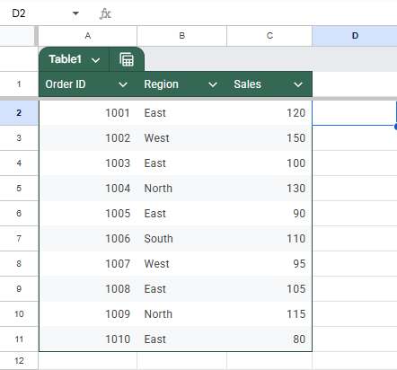
We’ll use the following example dataset where column B contains regions and column C contains sales figures:
Steps:
➤ Open your Google Sheet and click on the cell where you want the result to appear.
➤ Type the following formula:
=SUMIF(B2:B11, “East”, C2:C11).
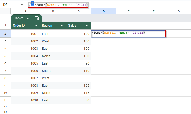
➤ Press Enter.
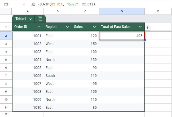
You’ll now see the total of all sales where the region is “East“. The result updates automatically if the data changes.
Use SUMIF to Sum if Cell Contains a Text Substring
When your target text may not be an exact match, for example, if the column includes values like “East Zone” or “North-East Region“, the regular SUMIF won’t work with plain criteria like “East“. In such cases, you can use wildcards with SUMIF to match partial text. The * wildcard tells Google Sheets to match any number of characters before or after the text you’re looking for.
Steps:
➤ Select the cell where you want the total to appear.
➤ Enter the formula:
=SUMIF(B2:B11, “*East*”, C2:C11)
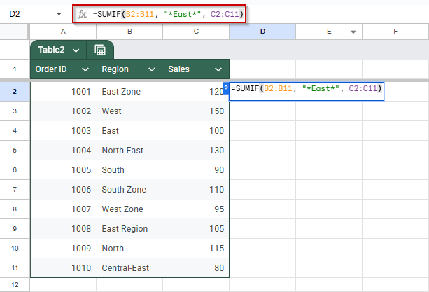
➤ Press Enter.
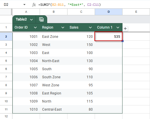
➤ You can replace “East” with any other keyword wrapped in asterisks to search for other partial matches (e.g., “*Zone*“).

Generate a Sum by Using SUMIFS for Multiple Conditions Including Text in Google Sheets
When you need to apply more than one condition while summing values in Google Sheets, the SUMIFS function is ideal. Unlike SUMIF, which handles a single condition, SUMIFS allows you to combine multiple criteria, for example, summing sales only if the region is “West” and the sales amount is greater than 1200. This method gives you more control and precision, especially in performance tracking or filtered reporting.
Steps:
➤ Click on the cell where you want the result to appear, for example, D2.
➤ Enter the following formula:
=SUMIFS(C2:C11, B2:B11, “West”, C2:C11, “>120”)
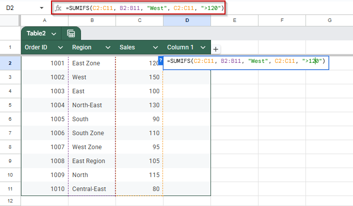
➤ Press Enter.
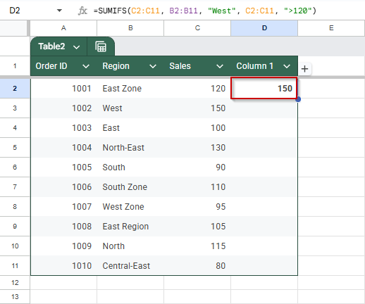
➤ The result will be the total sales from the West region, where each sale exceeds 120. You can adjust both conditions. For instance, you can change “West” to reference a cell (D1) or modify the sales threshold to suit your analysis.
Frequently Asked Questions
How do I sum cells if another cell contains specific text in Google Sheets?
Use =SUMIF(range, “text”, sum_range) to add values where corresponding cells match “text“. For partial matches, use wildcards like *text* for flexible criteria.
Can SUMIF work if the text is part of a longer string?
Yes. Use wildcards: =SUMIF(A2:A10, “*keyword*”, B2:B10) will sum values in B2:B10 where A2:A10 contains “keyword” anywhere in the cell.
How do I use SUMIF with a cell reference instead of hardcoded text?
Use =SUMIF(A2:A10, D1, B2:B10) where D1 contains your target text. This makes the formula dynamic and easier to update or reuse across different filters.
What’s the difference between SUMIF and SUMIFS?
SUMIF supports a single condition; SUMIFS handles multiple. For example, sum if Region = “West” and Sales > 1000: =SUMIFS(C2:C10, B2:B10, “West”, C2:C10, “>1000”).
Why is my SUMIF not working with text criteria?
Check for extra spaces or mismatched text cases. Use TRIM() or UPPER() function to normalize text. Also, ensure you’re not referencing merged or hidden cells improperly.
Wrapping Up
Using SUMIF and SUMIFS in Google Sheets makes it easy to calculate totals based on text criteria, whether you’re matching exact words, using cell references, or combining multiple conditions. These functions help keep your sheets organized and dynamic, allowing you to analyze key patterns without manual filtering.
As your datasets grow, mastering these conditional summing techniques will save you time and improve accuracy across all your reports.